Doing causal inference

Lab 04

GH classroom link

Link, submission Sep 19

Package installation

We use two packages that are not on CRAN but are quite useful. You can install them using either the devtools or remotes packages or using pak::pak. These are the touringplans and propensity packages.

remotes::install_github("LucyMcGowan/touringplans")
remotes::install_github("r-causal/propensity")
# devtools::install_github("LucyMcGowan/touringplans")
# devtools::install_github("r-causal/propensity")
# pak::pak("LucyMcGowan/touringplans")
# pak::pak("r-causal/propensity")

Building propensity score models

The propensity score is the probability of being in the exposed group, conditional on observed covariates.

• typically, we want to condition on potential confounders

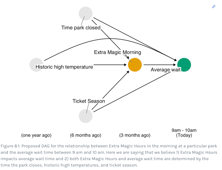
We will use some data on the Seven Dwarfs Mine train wait times at Disneyland to look at propensity scores. The question we want to address is, is there a relationship between whether there were “Extra Magic Hours” in the morning at Magic Kingdom and the average wait time for an attraction called the “Seven Dwarfs Mine Train” the same day between 9am and 10am in 2018? 

We first restrict the data to the 9am hour:

library(tidyverse)
library(broom)
library(touringplans)
seven_dwarfs_9am <- seven_dwarfs_train_2018 |> filter(wait_hour==9)

We will build a propensity score two ways: first by logistic regression and second by random forests

library(randomForest)
seven_dwarfs_ps_log <- glm(
  park_extra_magic_morning ~ park_ticket_season + park_close +  park_temperature_high, 
  data = seven_dwarfs_9am, 
  family = binomial
)

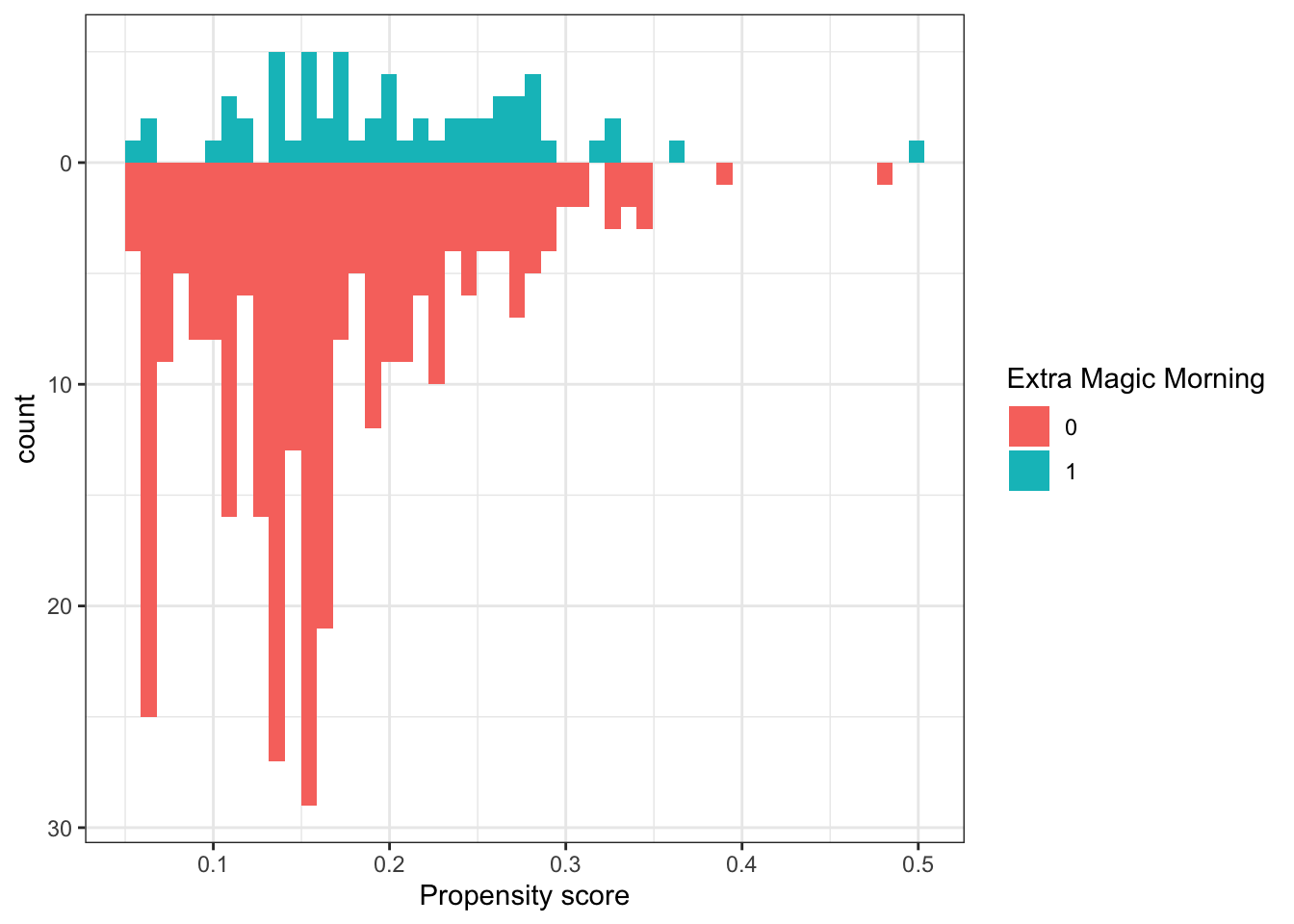
Let’s see what these propensity scores look like

seven_dwarfs_ps_log |> 
  augment(type.predict = 'response', data = seven_dwarfs_9am) |> 
  select(
    .fitted, park_date, park_extra_magic_morning, park_ticket_season, park_close, park_temperature_high
  ) |> head()

# A tibble: 6 × 6
  .fitted park_date  park_extra_magic_morning park_ticket_season park_close
    <dbl> <date>                        <dbl> <chr>              <time>    
1   0.302 2018-01-01                        0 peak               23:00     
2   0.282 2018-01-02                        0 peak               24:00     
3   0.290 2018-01-03                        0 peak               24:00     
4   0.188 2018-01-04                        0 regular            24:00     
5   0.184 2018-01-05                        1 regular            24:00     
6   0.207 2018-01-06                        0 regular            23:00     
# ℹ 1 more variable: park_temperature_high <dbl>

library(halfmoon)
seven_dwarfs_ps_log |> 
  augment(type.predict = 'response', data = seven_dwarfs_9am) |> 
  ggplot(aes(.fitted, fill = factor(park_extra_magic_morning)))+
    geom_mirror_histogram(bins=50)+
  scale_y_continuous(labels = abs)+
  labs(x = 'Propensity score', fill = 'Extra Magic Morning')+
  theme_bw()

Matching based on scores

library(MatchIt)
m <- matchit(
  park_extra_magic_morning ~ park_ticket_season + park_close + park_temperature_high,
  data = seven_dwarfs_9am
)
m

A matchit object
 - method: 1:1 nearest neighbor matching without replacement
 - distance: Propensity score
             - estimated with logistic regression
 - number of obs.: 354 (original), 120 (matched)
 - target estimand: ATT
 - covariates: park_ticket_season, park_close, park_temperature_high

matched_data = get_matches(m)
glimpse(matched_data)

Rows: 120
Columns: 18
$ id                       <chr> "5", "340", "12", "180", "19", "236", "25", "…
$ subclass                 <fct> 1, 1, 2, 2, 3, 3, 4, 4, 5, 5, 6, 6, 7, 7, 8, …
$ weights                  <dbl> 1, 1, 1, 1, 1, 1, 1, 1, 1, 1, 1, 1, 1, 1, 1, …
$ park_date                <date> 2018-01-05, 2018-12-17, 2018-01-12, 2018-07-…
$ wait_hour                <int> 9, 9, 9, 9, 9, 9, 9, 9, 9, 9, 9, 9, 9, 9, 9, …
$ attraction_name          <chr> "Seven Dwarfs Mine Train", "Seven Dwarfs Mine…
$ wait_minutes_actual_avg  <dbl> 33.0, 8.0, 114.0, 32.0, NA, NA, NA, NA, NA, N…
$ wait_minutes_posted_avg  <dbl> 70.55556, 80.62500, 79.28571, 52.22222, 75.00…
$ attraction_park          <chr> "Magic Kingdom", "Magic Kingdom", "Magic King…
$ attraction_land          <chr> "Fantasyland", "Fantasyland", "Fantasyland", …
$ park_open                <time> 09:00:00, 09:00:00, 09:00:00, 09:00:00, 09:0…
$ park_close               <time> 24:00:00, 23:00:00, 23:00:00, 22:00:00, 20:0…
$ park_extra_magic_morning <dbl> 1, 0, 1, 0, 1, 0, 1, 0, 1, 0, 1, 0, 1, 0, 1, …
$ park_extra_magic_evening <dbl> 0, 0, 0, 0, 0, 0, 0, 0, 0, 0, 0, 0, 0, 0, 0, …
$ park_ticket_season       <chr> "regular", "regular", "regular", "regular", "…
$ park_temperature_average <dbl> 43.56, 57.61, 70.91, 80.31, 50.07, 82.87, 62.…
$ park_temperature_high    <dbl> 54.29, 65.44, 78.26, 89.19, 64.04, 89.54, 73.…
$ distance                 <dbl> 0.18409891, 0.18380884, 0.15449940, 0.1547155…

Weighting

The idea is to weight each individual by \[w_{ATE} = \frac{X}{p} + \frac{1-X}{1-p}\]

library(propensity)
seven_dwarfs_wt <- seven_dwarfs_ps_log |> 
  augment(type.predict = 'response', data = seven_dwarfs_9am) |> 
  mutate(w_ate = wt_ate(.fitted, park_extra_magic_morning))

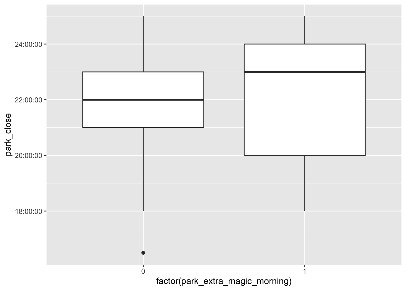
Evaluation

seven_dwarfs_wt |> 
  ggplot(aes(
    x = factor(park_extra_magic_morning),
    y = park_close,
    weight = w_ate
  )) + 
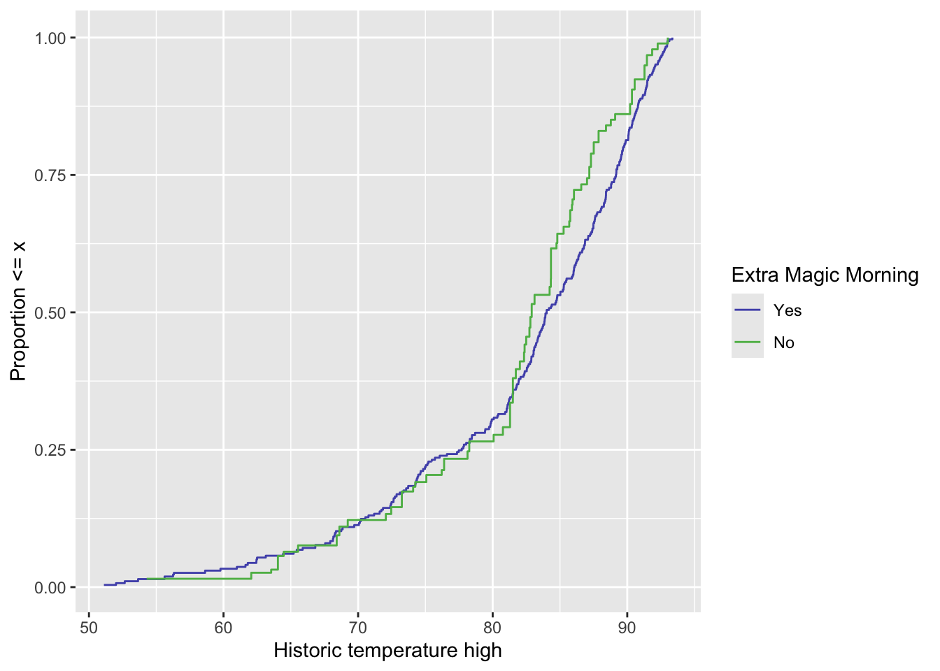
    geom_boxplot()

ggplot(
  seven_dwarfs_wt,
  aes(
    x = park_temperature_high,
    color = factor(park_extra_magic_morning)
  )
) +
  geom_ecdf(aes(weights = w_ate)) +
  scale_color_manual(
    "Extra Magic Morning",
    values = c("#5154B8", "#5DB854"),
    labels = c("Yes", "No")
  ) +
  labs(
    x = "Historic temperature high",
    y = "Proportion <= x"
  )

To do: repeat this analysis using a random forest model to generate the propensity scores