set.seed(3810)
library(tidyverse)
X <- rexp(10000, 1 / 5)
d <- tibble(x = sample(X, 50))Computational inference with R
Lab 1
Computational inference is the use of in silico methods, including resampling and Monte Carlo simulations, to make statistical inferences. The main tools that we will use here include the bootstrap and the permuation test
We will be using the packages rsample and infer for this.
Bootstrap confidence intervals
We can use the rsample package to do boostrap samples from data. We’ll start with a simulated population of 10000 subjects from a Exp(1/5) distribution, and then take a random sample of 50 who will be our study participants
Let’s first look at the distribution of x. We find that this is not distributed as a bell curve
hist(d$x)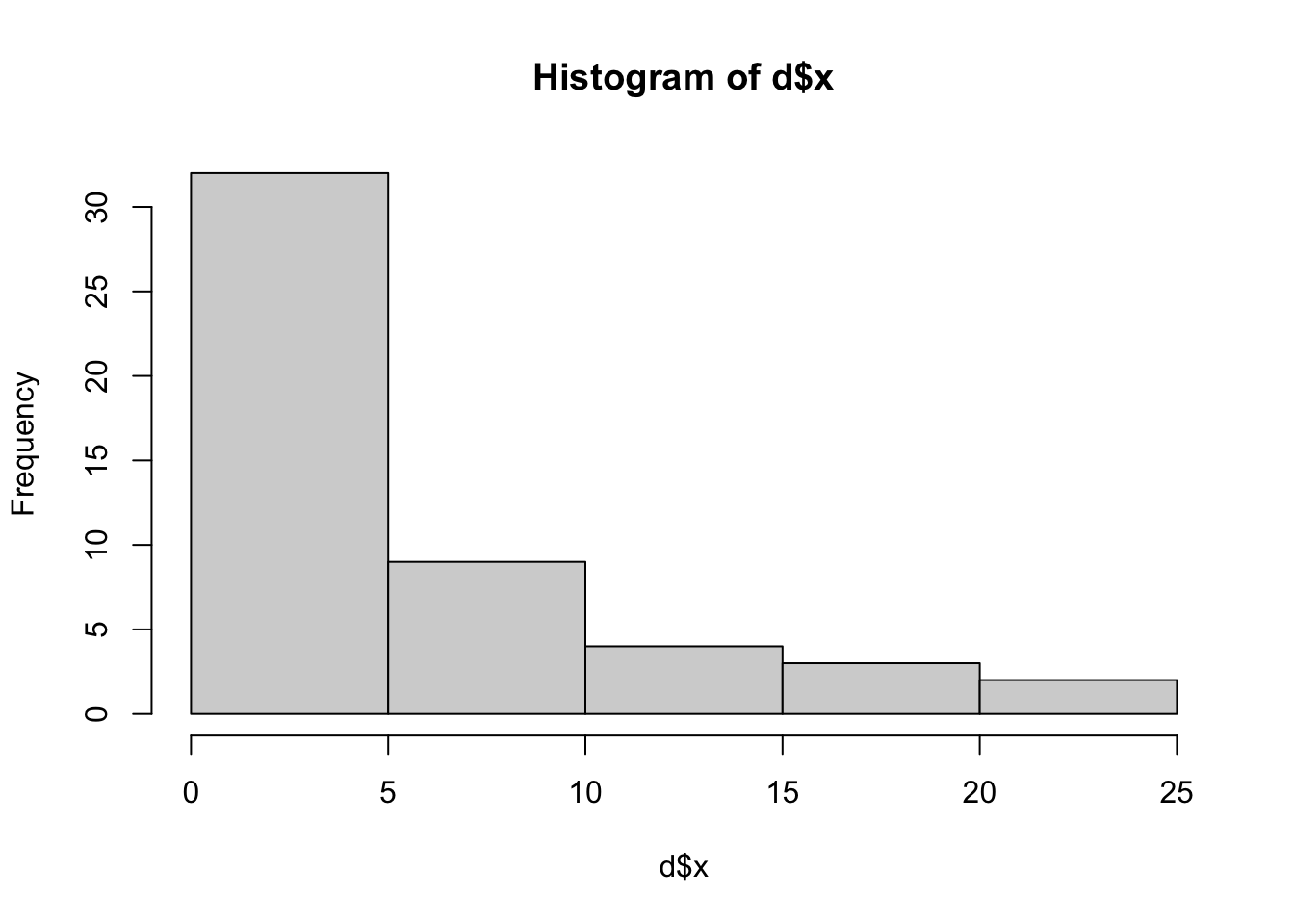
We’ll take 100 bootstrap samples from ths data and look at the distribution of the mean
library(rsample)
boots <- bootstraps(d, times = 1000)
boots
# Bootstrap sampling
# A tibble: 1,000 × 2
splits id
<list> <chr>
1 <split [50/19]> Bootstrap0001
2 <split [50/20]> Bootstrap0002
3 <split [50/17]> Bootstrap0003
4 <split [50/18]> Bootstrap0004
5 <split [50/18]> Bootstrap0005
6 <split [50/21]> Bootstrap0006
7 <split [50/19]> Bootstrap0007
8 <split [50/17]> Bootstrap0008
9 <split [50/15]> Bootstrap0009
10 <split [50/17]> Bootstrap0010
# ℹ 990 more rowsWe can now compute, and show, the bootstrap distribution of the mean
xbar <- map_dbl(boots$splits, \(d) mean(analysis(d)$x))
hist(xbar)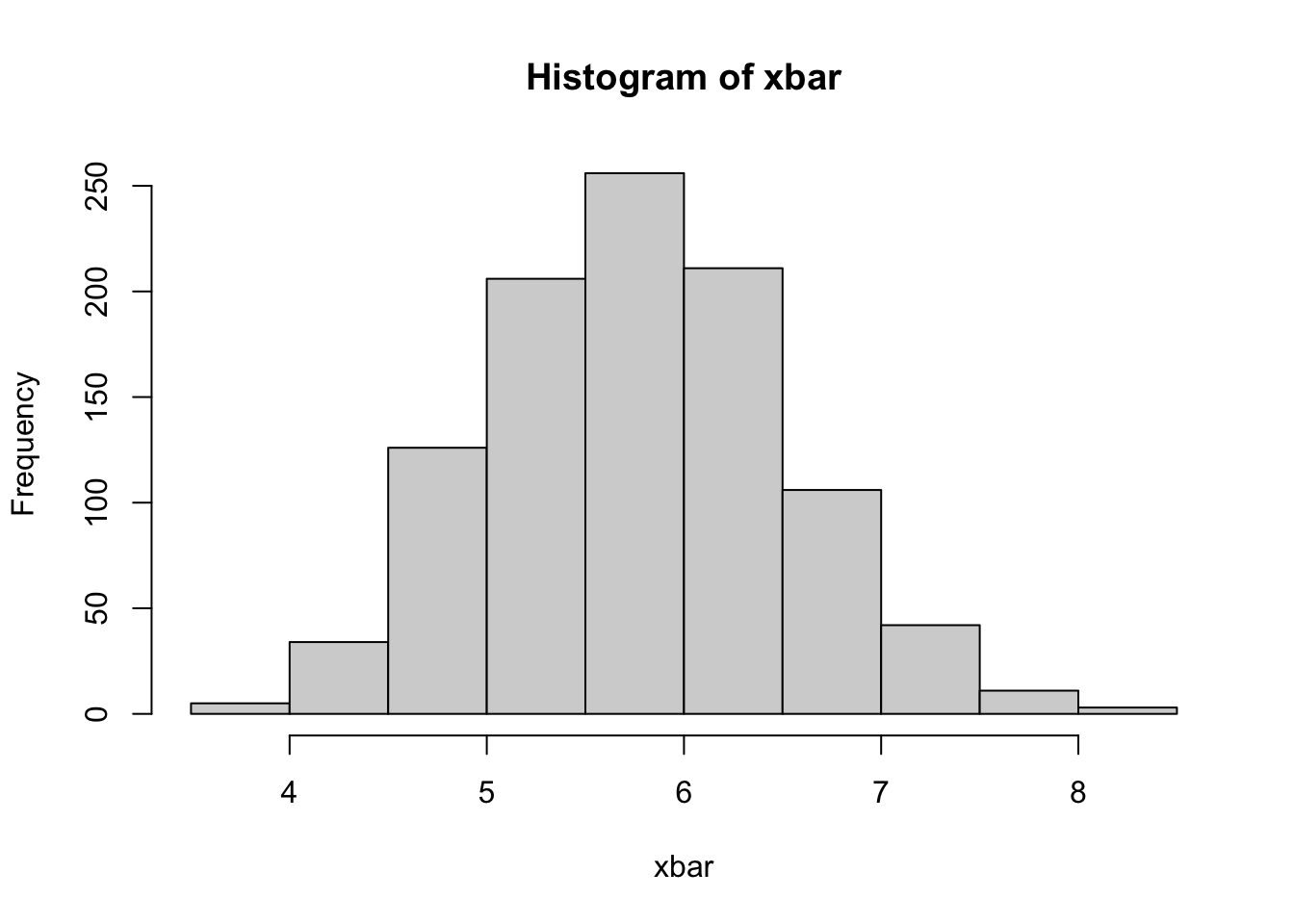
Let’s compare this to the sampling distribution of the mean, based on N=50
Xbar <- replicate(1000, mean(sample(X, 50)))
hist(Xbar)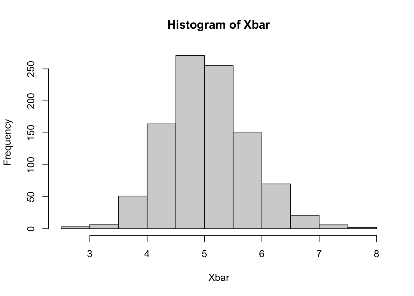
They actually look quite similar, which is what we’d expect. The bootstrap distribution centers around the mean of the sample, while the sampling distribution centers around the mean of the population, but otherwise they’re quite close. We can now compute a 95% confidence interval, and see how it compares with the theoretical confidence interval.
boot_ci <- quantile(xbar, c(0.025, 0.975))
asymp_ci <- t.test(d$x)$conf.int

boot_ci
2.5% 97.5%
4.334621 7.224055 asymp_ci[1] 4.258483 7.307741
attr(,"conf.level")
[1] 0.95So we have nice concordance.
But, with the bootstrap, we can compute confidence intervals for any computable statistic. Some of those might not have great theoretical confidence intervals. For example, we can do the bootstrap CI of the median
x_med <- map_dbl(boots$splits, \(d) median(analysis(d)$x))
hist(x_med)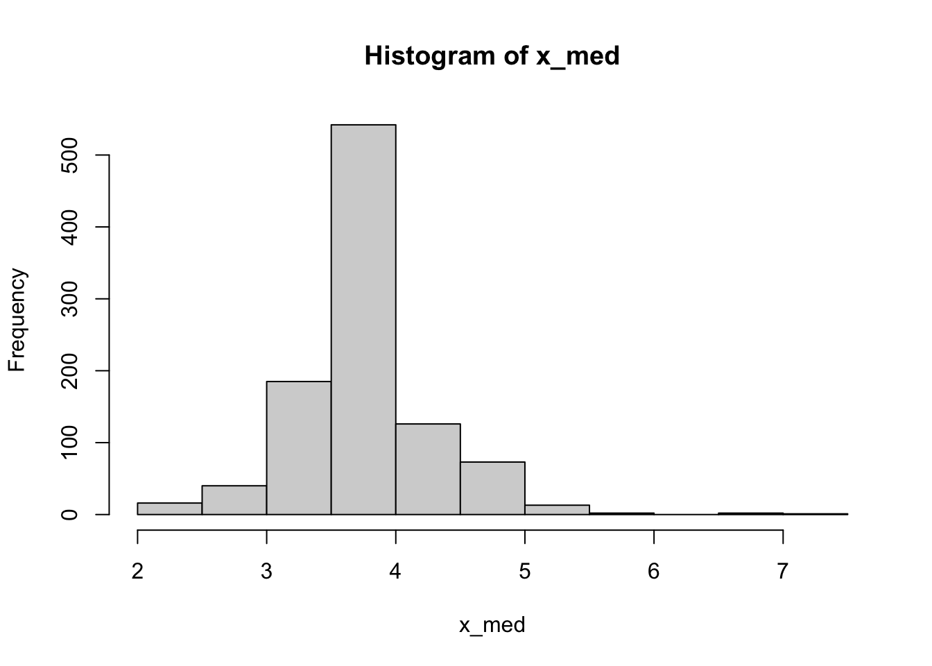
quantile(x_med, c(0.025, 0.975)) 2.5% 97.5%
2.782335 4.935429 or, for the 3rd quartile
x_q3 <- map_dbl(boots$splits, \(d) quantile(analysis(d)$x, 0.75))
hist(x_q3)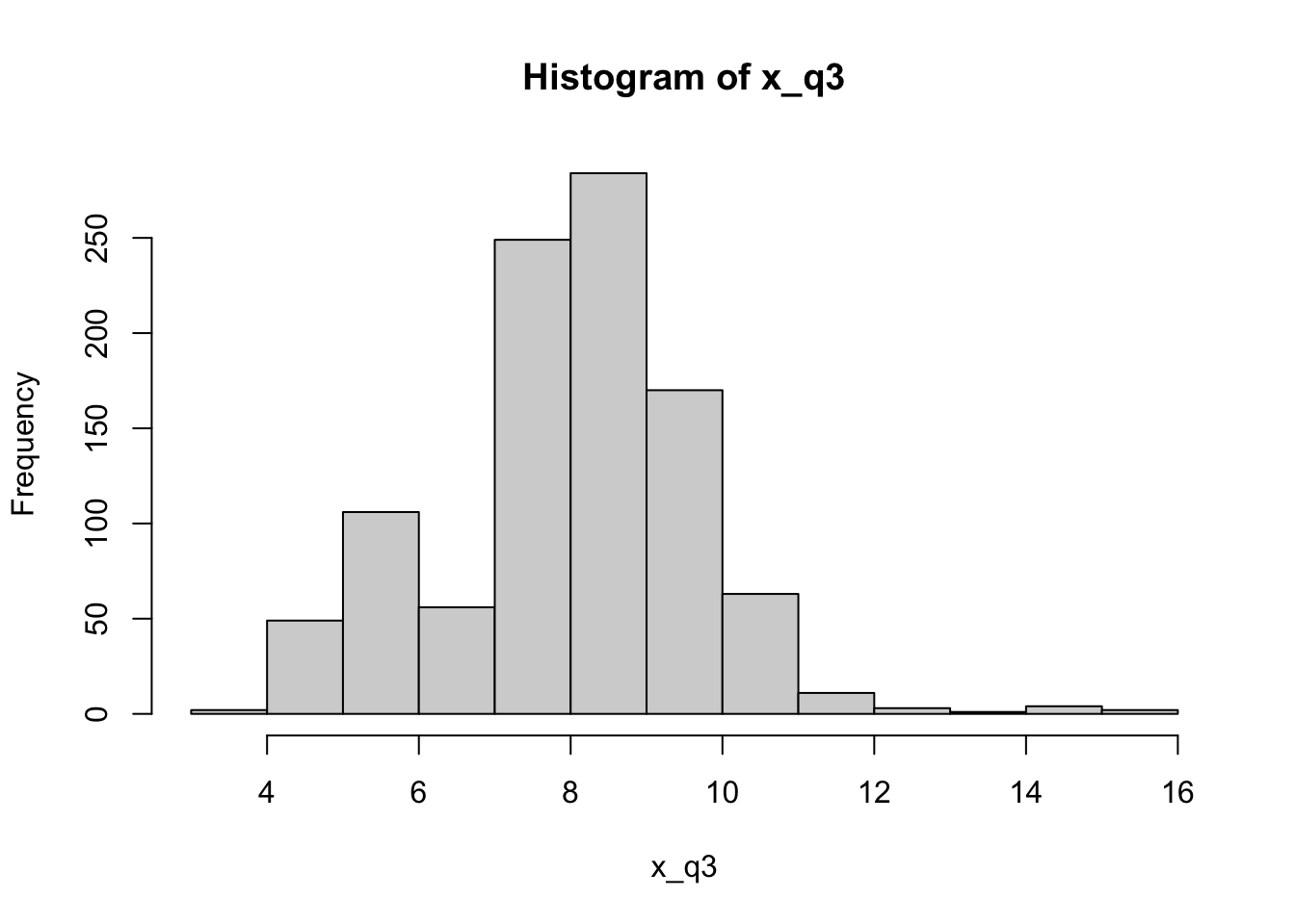
quantile(x_q3, c(0.025, 0.975)) 2.5% 97.5%
4.784135 10.500987 Hypothesis testing
Just like we saw above, we can do standard tests using resampling, specially permutation testing for 2-sample problems. Also, as earlier, the principle of permutation testing is more general and can be used to make inference about non-standard statistics like quantiles.
2-sample t-test
We will use the gss data to ask the question, do Americans work the same number of hours a week regardless of whether they have a college degree or not?
library(tidyverse)
library(infer)

ggplot(gss, aes(x = college, y = hours)) +
  geom_boxplot()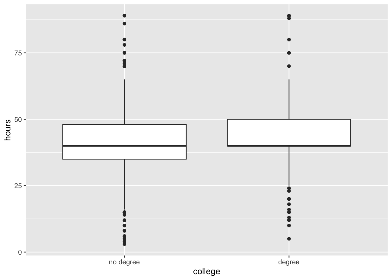
ggplot(gss, aes(x = hours, color = college)) +
  geom_density()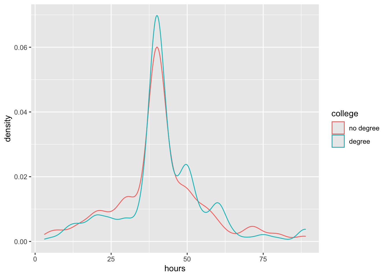
We use infer to first compute the test statistic (the t-statistic)
observed_stat <- gss |>
  specify(hours ~ college) |>
  calculate(stat = "diff in means", order = c("degree", "no degree"))
observed_stat
Response: hours (numeric)
Explanatory: college (factor)
# A tibble: 1 × 1
stat
<dbl>
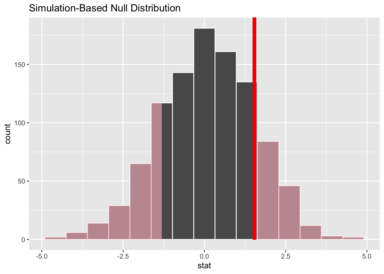
1 1.54Now we compute the null distribution under the assumption of no difference, using permutations
# generate the null distribution with randomization
null_dist_2_sample <- gss |>
  specify(hours ~ college) |>
  hypothesize(null = "independence") |>
  generate(reps = 1000, type = "permute") |>
  calculate(stat = "diff in means", order = c("degree", "no degree"))

# visualize the randomization-based null distribution and test statistic!
null_dist_2_sample |>
  visualize() +
  shade_p_value(observed_stat,
    direction = "two-sided"
  )
How about trying the exponential distribution
set.seed(1038)

d <- tibble(
  x = c(rexp(100, 1), rexp(100, 2)),
  grp = factor(c(rep("A", 100), rep("B", 100)))
)

observed_stat <- d |>
  specify(x ~ grp) |>
  calculate("diff in means")
observed_stat
Response: x (numeric)
Explanatory: grp (factor)
# A tibble: 1 × 1
stat
<dbl>
1 0.537ggplot(d, aes(x, color = grp)) +
geom_density()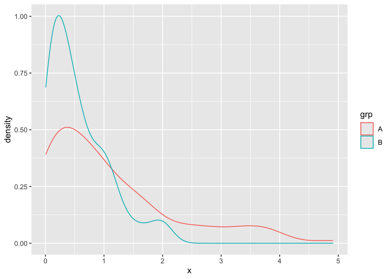
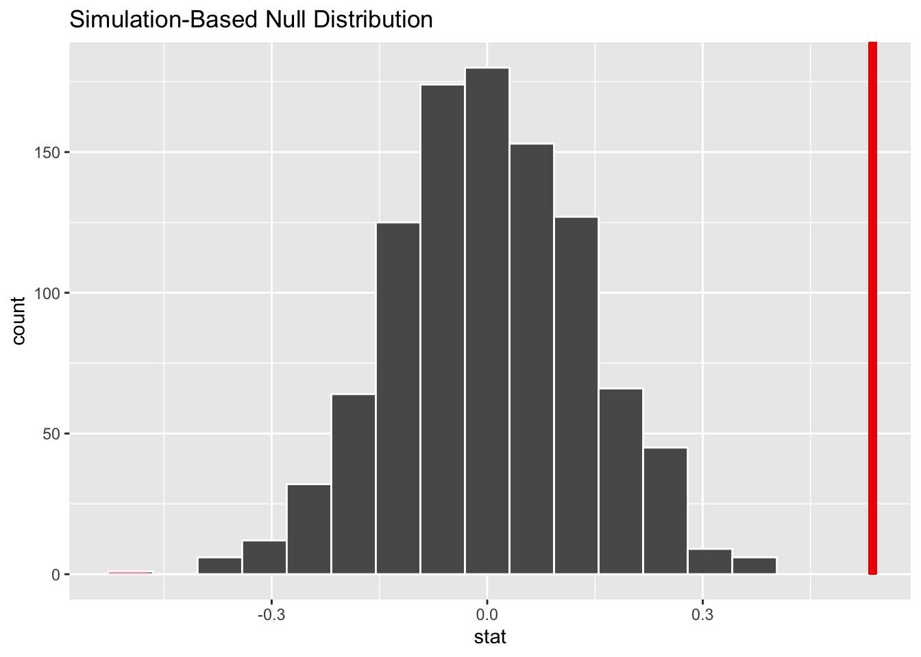
null_dist <- d |>
  specify(x ~ grp) |>
  hypothesize(null = "independence") |>
  generate(reps = 1000, type = "permute") |>
  calculate("diff in means")

null_dist |>
  visualize() +
  shade_p_value(observed_stat,
    direction = "two-sided"
  )
null_dist |>
  get_p_value(
    obs_stat = observed_stat,
    direction = "two-sided"
  )
# A tibble: 1 × 1
p_value
<dbl>
1 0Let’s contrast this with usual tests
t.test(x ~ grp, data = d)
    Welch Two Sample t-test

data:  x by grp
t = 4.4414, df = 138.66, p-value = 1.812e-05
alternative hypothesis: true difference in means between group A and group B is not equal to 0
95 percent confidence interval:
 0.2976781 0.7753861
sample estimates:
mean in group A mean in group B
1.0987545 0.5622223 wilcox.test(x ~ grp, data = d)
    Wilcoxon rank sum test with continuity correction

data:  x by grp
W = 6335, p-value = 0.001111
alternative hypothesis: true location shift is not equal to 0set.seed(1004)
nsim <- 100
n <- 10
p_t <- rep(0, nsim)
p_w <- rep(0, nsim)
p_perm <- rep(0, nsim)
for (i in 1:nsim) {
d <- tibble(
x = c(rexp(n, 1), rexp(n, 1.5)),
grp = factor(c(rep("A", n), rep("B", n)))
)
p_t[i] <- t.test(x ~ grp, data = d)$p.value
p_w[i] <- t.test(x ~ grp, data = d)$p.value
obs_stat <- d |>
specify(x ~ grp) |>
calculate("diff in means")
null_dist <- d |>
specify(x ~ grp) |>
hypothesize(null = "independence") |>
generate(reps = 1000, type = "permute") |>
calculate("diff in means")
p_perm[i] <- null_dist |>
get_p_value(
obs_stat = obs_stat,
direction = "two-sided"
) |>
pull(p_value)
}
mean(p_t < 0.05)
mean(p_w < 0.05)
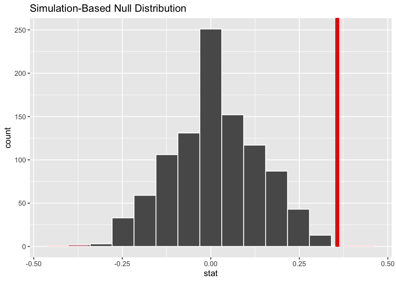
mean(p_perm < 0.05)We can also do a test for the median, using the permutation approach
observed_stat <- d |>
  specify(x ~ grp) |>
  calculate("diff in medians")

null_dist <- d |>
  specify(x ~ grp) |>
  hypothesize(null = "independence") |>
  generate(reps = 1000, type = "permute") |>
  calculate("diff in medians")

null_dist |>
  visualize() +
  shade_p_value(observed_stat,
    direction = "two-sided"
  )
You can also compute the bootstrap confidence interval using infer
d |>
  filter(grp == "A") |>
  specify(response = x) |>
  calculate(stat = "median")
Response: x (numeric)
# A tibble: 1 × 1
stat
<dbl>
1 0.769d |>
filter(grp == "A") |>
specify(response = x) |>
generate(reps = 1000, type = "bootstrap") |>
calculate(stat = "median") |>
get_ci()# A tibble: 1 × 2
lower_ci upper_ci
<dbl> <dbl>
1 0.629 0.964The theoretical median is 0.6931472, for comparison.