Lecture 9

Bayesian analysis

Abhijit Dasgupta

Georgetown University

Fall 2024

Agenda and goals for the day

Lecture

The two paradigms (frequentist and Bayesian)
Decisions from a Bayesian perspective
Usefulness and examples for statistical inference

Lab

Basics of Bayesian computation
Fitting models using Bayesian principles
Pointers to more advanced computations

The two paradigms

Frequentists see probability as long-term frequencies

The underlying idea in frequentist frameworks is that one can observe a phenomenon repeatedly over time and establish the distribution of the outcome of interest

In reality, we utilize idealized models (Binomial, Normal, etc) to model these “long term” probabilities

The practice is based on the concept of multiple repetitions of the same experiment and what might happen

Tools of the trade

The central limit theorem

This says that, as you take larger and larger samples, the distribution of the sample mean, over repeated identical experiments, will look like a normal distribution

Theorem

Let \(X_1,\dots,X_n\) are independent and identically distributed with mean \(\mu\) and variance \(\sigma^2\), then

\[ \sqrt{n}(\bar{X_n} - \mu)/\sigma \rightarrow^d N(0,1) \]

Tools of the trade

The weak law of large numbers (WLLN)

Theorem

Let \(X_1,\dots,X_n\) be independent and identically distributed random variables with mean \(\mu\) and variance \(\sigma^2\). Then the sample mean \(\bar{X_n}\) goes in probability to the population mean \(\mu\) as \(n \rightarrow \infty\).

\[ \Pr (|\bar{X_n} - \mu | > \epsilon) \rightarrow 0 \quad \text{as } n\rightarrow\infty \]

Tools of the trade

Null hypothesis significance testing (NHST)

We postulate a null hypothesis \(H_0\) and an alternative hypothesis \(H_1\). We devise a statistical test \(\phi(X)\) that attempts to judge when the data provides sufficient evidence to favor \(H_1\) over \(H_0\) (which is often a strawman). This test can only reject \(H_0\). The test \(\phi(X)\) takes values 1 (reject \(H_0\)) and 0 (does not reject \(H_0\)).

The test \(\phi(X)\) can incur two kinds of errors:

Type I error: P((X) = 1 | \(H_0\) is true)
Type II error: P((X) = 0 | \(H_0\) is false)

We also will see another quantity, statistical power of a test, which is defined as 1 - Type II error, i.e., P((X) = 1 | \(H_0\) is false)

Tools of the trade

Null hypothesis significance testing (NHST)

The Neymann-Pearson paradigm of NHST states that we fix the Type I error at some number \(\alpha\), and proceed to find that optimal test \(\phi(X)\) that maximizes the statistical power, i.e., minimizes the Type II error, usually denoted by \(\beta\).

For simple hypothesis, such a test is generally of the form

\[ \phi (X) = \left\{\begin{array}{ll} 1& T(X) \geq c\\ 0 & T(X) < c \end{array} \right. \]

for some test statistic T(X) and some number \(c\), where \(c\) is determined by the value of \(\alpha\).

Example

The one-sample test for the mean, \(H_0: \mu = \mu_0\) vs \(H_1: \mu \neq \mu_0\) rejects the null hypotheses if

\[ |\sqrt{n}(\bar{X_n} - \mu_0)/s| > z_{1-\alpha/2} \]

Tools of the trade

Null hypothesis significance testing (NHST)

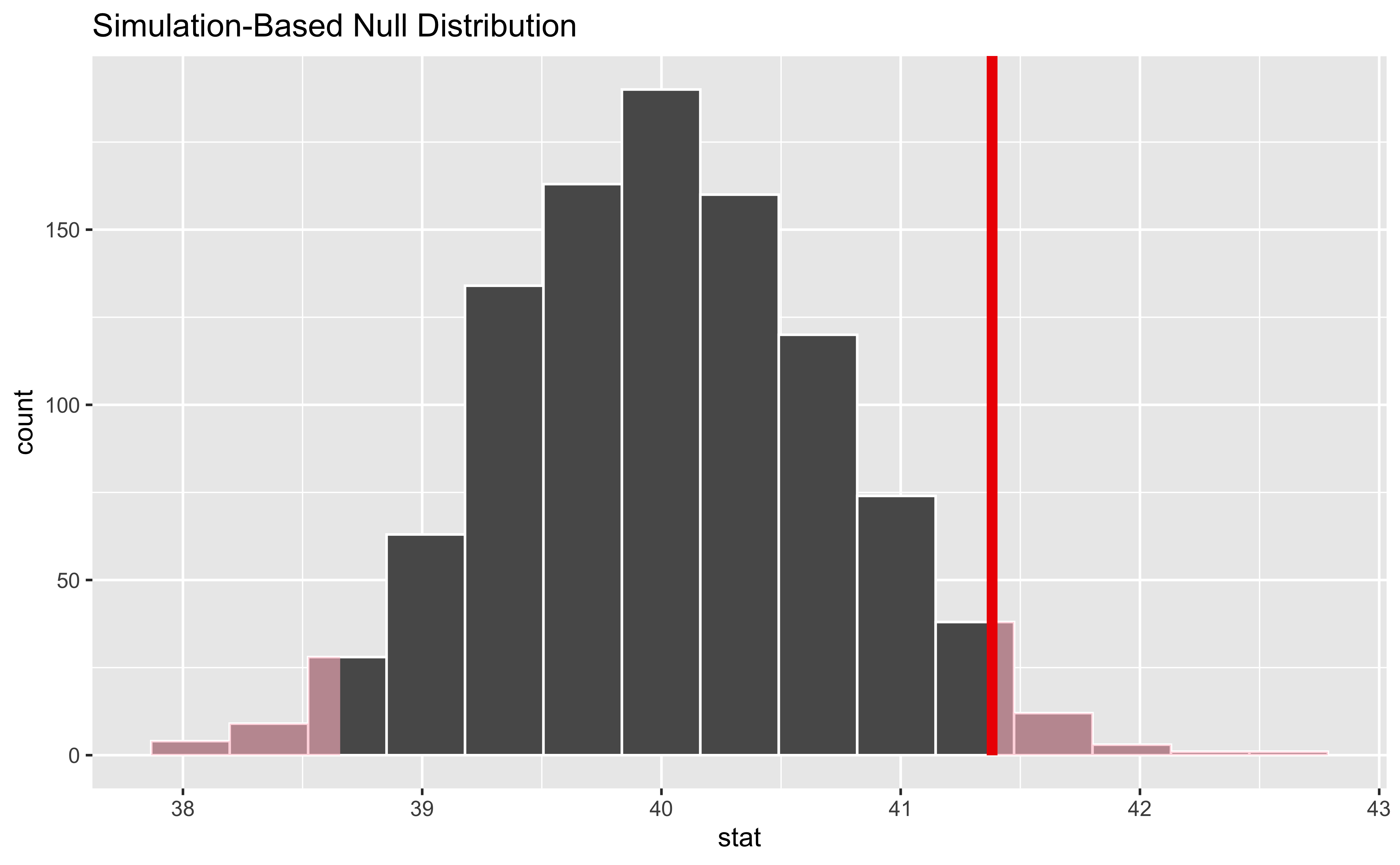
The p-value gives the probability, under \(H_0\) of seeing an observation at least as extreme as the one we observed

Note, this is based on the idea of repeated identical experiments

For most statistical tests, the observed value of the test statistic is compared to quantiles of the (idealized) sampling distribution (often the normal distribution due to the CLT) to get the p-value

Tools of the trade

Confidence intervals

We assume that there is a true value of a parameter \(\theta\).

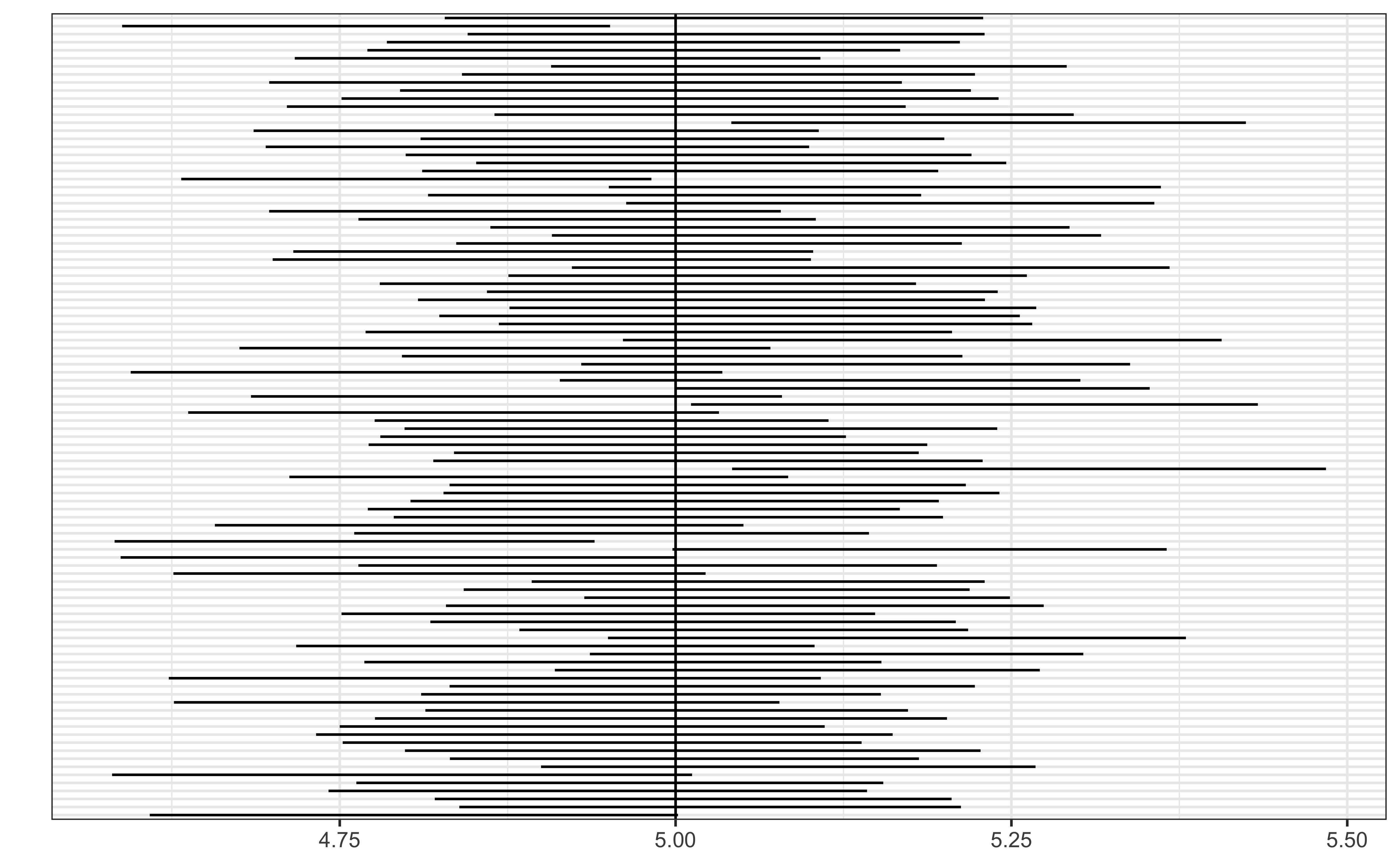
We specify a number \(0<\alpha<1\) and define a bivariate statistic (L(X), U(X)) so that, over repeated random samples of the same size from the underlying population, the computed interval from L(X) to U(X) will miss the true value of \(\theta\) in \(100\alpha\) % of the samples.

Warning

What is random in a confidence interval is the actual computed interval!!

Confidence intervals are almost always misinterpreted to mean that “there is a 95% chance that the true parameter falls within the interval”, rather than “95% of the time, intervals constructed in this manner will cover the true parameter”

Tools of the trade

Confidence intervals

Pitfalls of the frequentist approach

All arguments are based on non-observable “repeated experiments” rather than solely based on the data at hand
The p-value, which is the basis of much inference, is based on the assumption that \(H_0\) is true, which is unverifiable. It is saying that, if we assume that, how unlikely are we to see what we’re seeing. It also just says that, so we can’t actually infer that the alternative \(H_1\) is more plausible (ever!!) or “correct”, or what kinds of \(H_1\) would have the data at hand be more plausible.
The p-value by itself is not very useful without the domain context, and the corresponding effect size. Recall that the p-value is just an indication of the signal-to-noise ratio in the data, and so with very precise data, even a very small signal can have a small p-value
The need for preserving overall Type I error results in the need for multiple comparisons corrections (essentially reducing the p-value threshold on a per-test basis), but also results in significant loss of power and hence loss of detectable signals
The confidence interval is very frequently mis-interpreted as the chance that the true value of \(\theta\) lies in the interval is \(100(1-\alpha)\)%. As we shall see, this is the interpretation of the Bayesian credible interval

Bayesian statistics:
A different approach

What is Bayesian analysis?

A Bayesian analysis is a particular approach of using probabilities to answer statistical problems

What question should we ask our data to inform decision making?

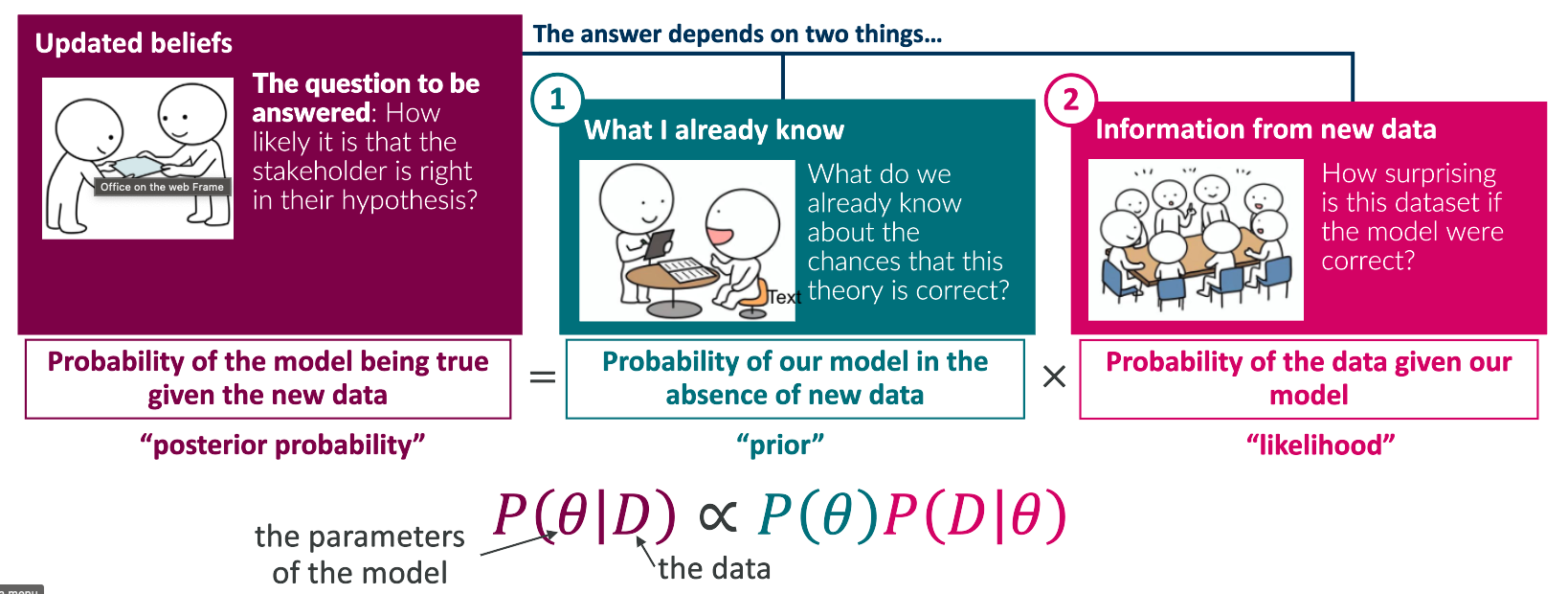
“Given the data and everything I already know, what are the chances that my hypothesis is correct?”

This is the question that a Bayesian analysis answers

What question should we ask our data to inform decision making?

It is well-established and convenient to ask this question:

“What is the chance of getting this data if my null hypothesis is true?”
(or “what is the p-value?”)

A Bayesian analysis asks and can answer the question:

“Given the data and everything I already know, what are the chances that my hypothesis is correct?”

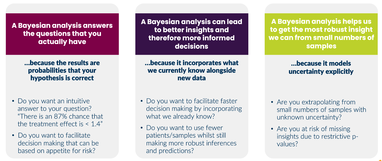
There are many advantages to framing the question in a Bayesian way that can help us make faster and more robust decisions

What is Bayesian analysis?

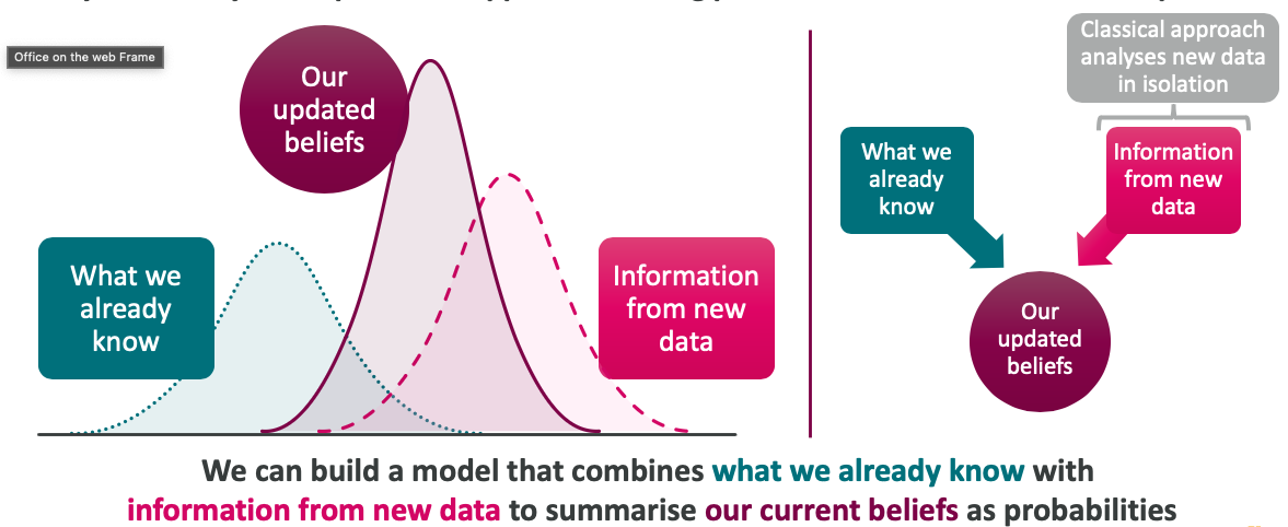
Bayesian analysis answers our questions as fully as possible by incorporating everything we know

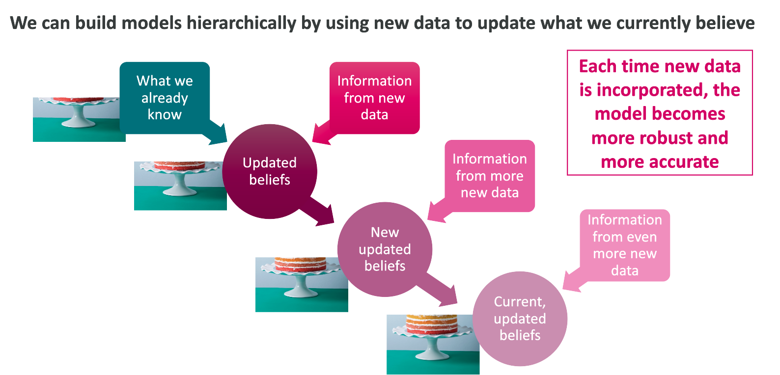
An example: I left my last piece of birthday cacke in the fridge. I suspect this waws a bad idea as my partner is working form home today. I am worried that she will eat my cake. I get back from work to discover icing, and a guilty look, on her face

Bayesian analysis answers our questions as fully as possible by incorporating everything we know

Another example: A stakeholder has a theory and has just acquired some new data that might support that theory – they want to know the chances that their theory is correct in light of this new data.

When should we consdier a Bayesian approach?

A Bayesian analysis can facilitate faster, more informed decision making with known risk profiles

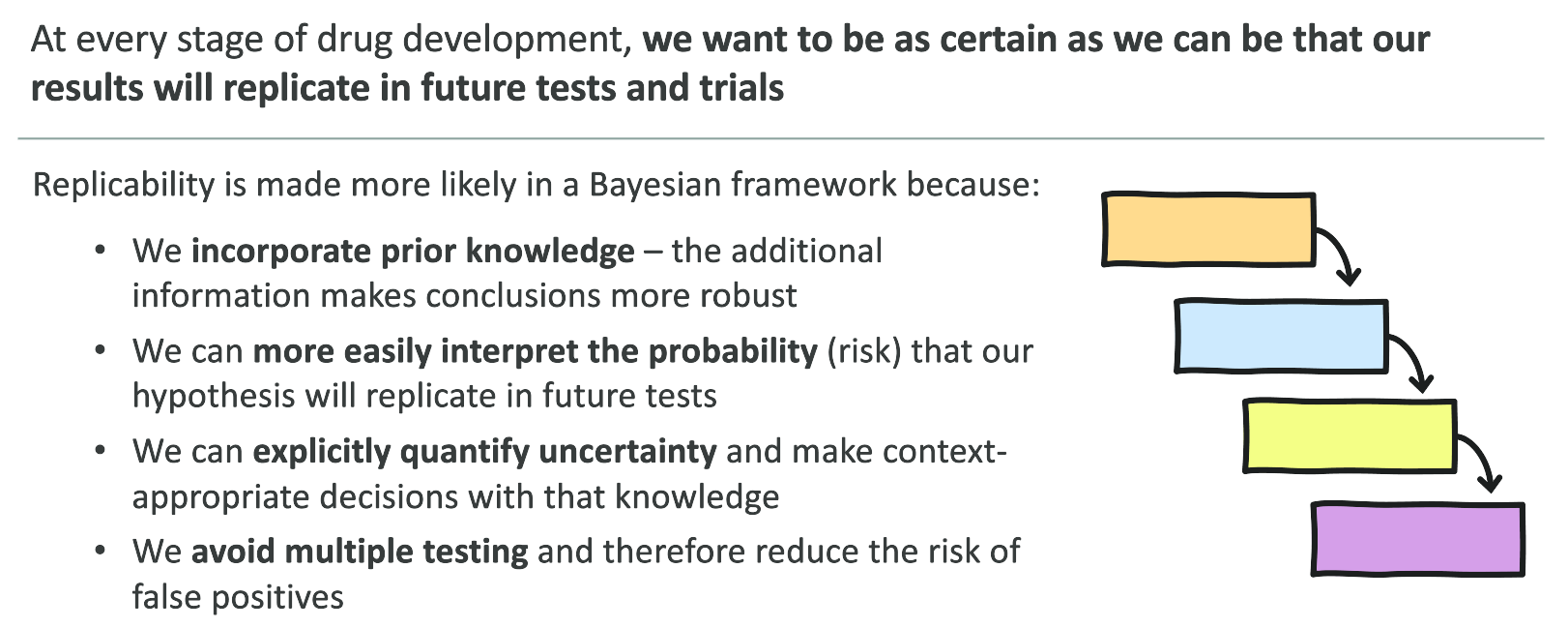
A Bayesian approach can improve replicability

Bayesian analysis allows us to update our beliefs over time

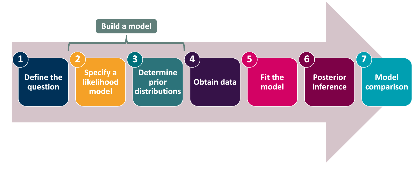
How is a Bayesian analysis implemented?

The Bayesian framework

The parameter of interest \(\theta\) is treated as a variable, not a constant.
\(\theta\) is a random variable with a distribution denoted by \(p(\theta)\), called the prior distribution

The data \(D = X_1,\dots,X_n\) comes as i.i.d. data from a data model defined by a probability distribution \(p(D|\theta)\) dependent on \(\theta\).
The p.d.f./p.m.f of this distribution, defined as a function of the data, is called the likelihood \(L(\theta | D)\).

The posterior distribution can be computed as

\[ p(\theta | D) \propto p(\theta) p(D | \theta) \]

Why do we have the \(\propto\)?

Bayesian inference

Bayesian inference is entirely based on the posterior distribution \(p(\theta | D)\)

We can ask and quantify questions like \(P(\theta \in (-1, 1) | D)\), \(P(\theta > 2| D)\), …
Inference becomes an estimation problem
We can compute credible intervals (CR) from \(P(\theta \in CR | D) = 0.95\)

We can actually quantify the chance that a hypothesis is true.

If \(H_0: \theta \in\Theta_0\) vs \(H_1: \theta \in \Theta_1\) then we can compute

\[ P(\theta \in \Theta_0 | D), \quad P(\theta\in\Theta_1 | D) \]

CONTROVERSY: The prior distribution

To get to the posterior, one must first define a prior distribution \(p(\theta)\) for the parameters of interest

This has been one of the most controversial parts of the Bayesian method
Critics have said that the specification of the prior makes the process subjective, which can bias our inference
- We “should be completely agnostic”, which is what frequentist methods appear to be

We are rarely completely ignorant about values a parameter can take
Domain knowledge often dictates the prior distribution
“Priors are never arbitrary” but can be justified by domain knowledge (Richard McElreath, 2023)
The frequentist method corresponds often to the assumption of a uniform distribution as a prior. This too, is a choice.

The prior distribution

The prior distribution theoretically can be elicited from expert opinion and knowledge as well as prior data. This is a process.

We will often choose prior distributions based on heuristic considerations of the constraints a parameter will be under
There is a choice of priors, called conjugate priors, for a particular data model (likelihood function), so that using those priors results in the posterior being in the same family as the prior
- One can get analytic solutions to the posterior

Conjugate priors

If you have a binary (yes/no) variable that you are observing, and you’re interested in the probabilty of a “yes”, taking the prior as a Beta distribution results in a Beta posterior.

\[ \theta \sim Beta(\alpha,\beta)\\ X_1, \dots, X_n \sim Bin(1, \theta) \] then \[ \theta | X \sim Beta(\alpha + \sum X, \beta + n - \sum X) \]

The parameters \(\alpha, \beta\) are called hyperparameters.

Hyperparameters can have priors, too

Conjugate priors

If our data comes from a \(N(\mu, \sigma^2)\) distribution with known \(\sigma\), then

\[ \mu \sim N(\mu_0, \sigma_0^2)\\ X_1,\dots,X_n \sim N(\mu,\sigma^2) \]

then

\[ \mu | X_1,\dots,X_n \sim N\left(\frac{1}{\frac{1}{\sigma_0^2}+\frac{1}{\sigma^2}} \left( \frac{\mu_0}{\sigma_0^2} + \frac{\sum X}{\sigma^2}\right), \frac{1}{\sigma_0^2} + \frac{n}{\sigma^2} \right) \]

Tip

A list of conjugate priors is given here

Prior predictive checks

We want to see if our choice of prior leads to data that is reasonably what we would expect. This is called a prior predictive check, and is achieved by generating data based on the prior choice.

Computing the posterior

With a conjugate prior, computing the posterior distribution is analytic.

Let us consider the beta-binomial conjugate family, with a \(Beta(1,1)\) prior

Play around with how much data is needed to move the ticker on our knowledge of \(p\).

Bayes factor

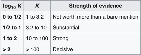
The Bayes factor is the relative evidence for different models (or different parameter sets under the same model) given the data

\[ k = \frac{P(\Theta_1 | D)}{P(\Theta_2 | D)} \]

Kass & Raftery (2005) provided a rule of thumb when evaluating Bayes factors

An example

We’re interested in evaluating an assay to see if it is sensitive enough for our purposes. We deem an assay to be acceptable if it has sensitivity of 95% or above. It is considered unacceptable if the sensitivity is below 90%.

We run the test on 100 sick people and get 95 positive tests.

The model

\[ \theta \sim Beta(4,1)\\ X \sim Bin(100, \theta) \]

Under this conjugate prior, the posterior distribution of \(\theta\) is Beta(4 + X, 1 + 100 - X).

Lecture 9

Agenda and goals for the day

Lecture

Lab

The two paradigms

Frequentists see probability as long-term frequencies

Tools of the trade

The central limit theorem

Tools of the trade

The weak law of large numbers (WLLN)

Tools of the trade

Null hypothesis significance testing (NHST)

Tools of the trade

Null hypothesis significance testing (NHST)

Tools of the trade

Null hypothesis significance testing (NHST)

Tools of the trade

Confidence intervals

Tools of the trade

Confidence intervals

Pitfalls of the frequentist approach

Bayesian statistics: A different approach

What is Bayesian analysis?

What question should we ask our data to inform decision making?

What question should we ask our data to inform decision making?

What is Bayesian analysis?

Bayesian analysis answers our questions as fully as possible by incorporating everything we know

Bayesian analysis answers our questions as fully as possible by incorporating everything we know

When should we consdier a Bayesian approach?

A Bayesian analysis can facilitate faster, more informed decision making with known risk profiles

A Bayesian approach can improve replicability

Bayesian analysis allows us to update our beliefs over time

How is a Bayesian analysis implemented?

The Bayesian framework

Bayesian inference

CONTROVERSY: The prior distribution

The prior distribution

Conjugate priors

Conjugate priors

Prior predictive checks

Computing the posterior

Bayes factor

An example

The model

An example

Prior predictive checks

An example

Resources

Bayesian statistics:
A different approach