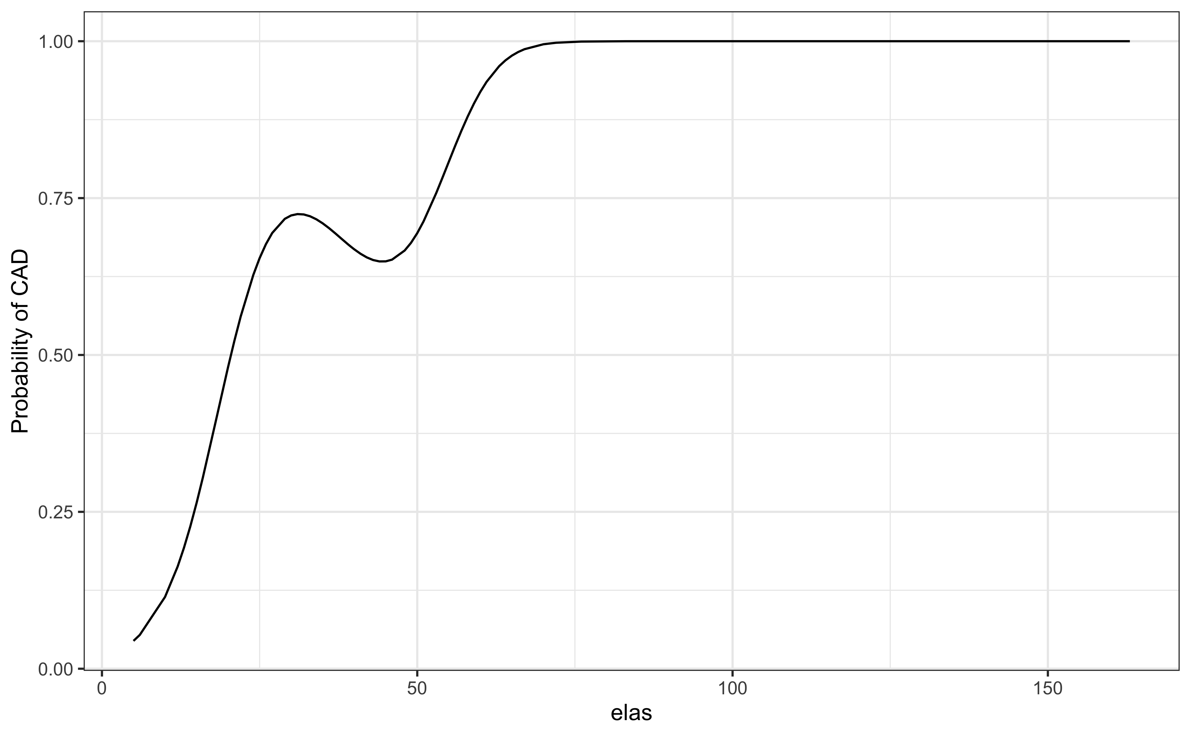
library(tidyverse)
library(tidymodels)
library(rms)

data(elas, package="OptimalCutpoints")

model <- glm(status ~ rcs(elas), data = elas, family = binomial)
a <- augment(model, newdata=elas, type.predict = 'response')
ggplot(a, aes(elas, .fitted))+geom_line()+theme_bw()+
labs(y = "Probability of CAD")Lecture 8
Biomarker Discovery
Georgetown University
Fall 2024
Agenda and goals for the day
Lecture
What is a biomarker?
Biomarker discovery
Dichotomania
Lab
- Multiple testing correction
- Penalized regression
Class logistics
Deadlines
- Survival homework due Monday, October 28
- High-dimensionsal/Biomarker homework due Sunday, Nov 3
Upcoming attractions
- Introduction to Bayesian modeling and analysis
- Machine learning applications
- How many subjects for a study?
What is a biomarker?
A possible definition
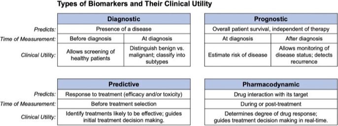
A biological marker (biomarker) can be defined as a characteristic that is measured as an indicator of normal or pathogenic processes (prognosis), or biological response to an exposure or intervention (predictive). There are other definitions based on clinical utility.
What is a biomarker?
Normally collected
- Diastolic blood pressure
- BMI
- HbA1C (for diabetes)
- C-reactive protein (for inflammation)
- LDL and HDL cholesterol, triglycerides
- ALT and AST (for liver function)
- Prostate-specific antigen (PSA, for prostate cancer)
- EKG
- Imaging
Specialized
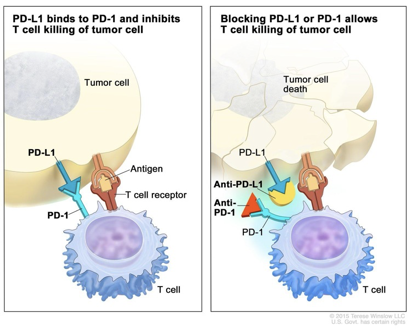
- PD-1/PD-L1, CTLA-4 (cancer drug targets, immune checkpoint inhibitors)
- BRCA 1/2 (gene for breast, ovarian, prostate cancer)
- ER, PR, HER2 (prognostic/predictive for breast cancer and Tx)
- EGFR (for lung cancer)
- ctDNA (circulating tumor DNA) for risk modeling, drug efficacy and early detection of recurrence
- Troponin (for acute coronary syndrome)
- Serum creatinine (for kidney health)
The search for reliable biomarkers
We want to identify small numbers (or perhaps singletons) of biomarkers that are prognostic or predictive in the clinical setting
From a data science perspective:
- The effect should be robust (should not be a false positive)
- The effect should be reproducible in new but similar data
Technology now offers us high-throughput, multiplexed solutions to generate candidates. What is the best way of taking advantage of this?
We have too many candidates and not enough observations
Problems
Selection: these candidates are likely to be highly correlated, meaning that the information provided by any one of them is contained among some of the other ones
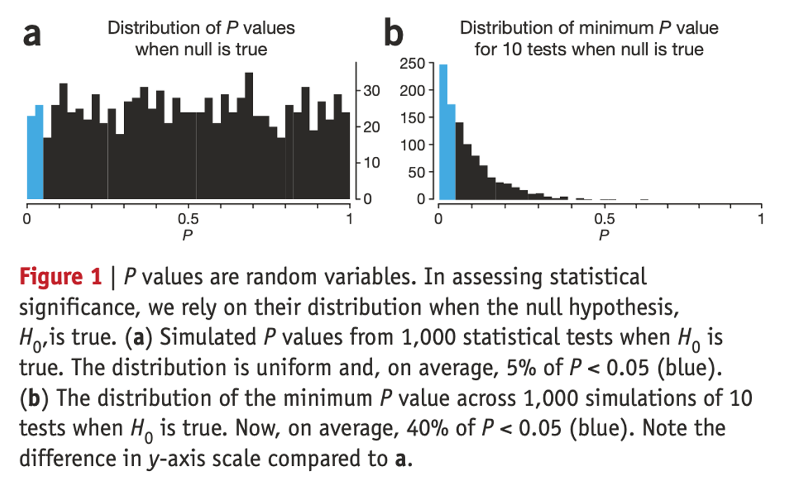
Reproducibility: we may need to perform so many tests that we are guaranteed to find statistically significant results at most common p-value levels (0.05, 0.01, 10-50), even when there are not real predictive biomarkers. On its own, a small p value is not evidence for anything**
Robustness of identification: small changes in the training or testing data set could lead to another (equally unreliable) biomarker proposal.
Non-optimal design: if data come from a source that was not experimentally designed for biomarker selection, we lose some statistical guarantees that makes the robustness of the results harder to establish.
When working with any data source, appropriate data beats lots of data
Use your prior knowledge and experience!
- Be clear about what you know beforehand:
- Group, a priori, your thoughts
- There is strong a priori evidence for ADSF2 and PQRS1
- There is weak a priori evidence for QWERTY1, ZXCV3, UIOP5, …, up to about 20.
- There is little evidence for anything else
- Group, a priori, your thoughts
- This will help you interpret what you find. Explanations after the fact are irrelevant: people are good at telling stories.
- Go back to first principles:
- Since theory is insufficient, compare your biomarkers’ predictivity with the biomarkers’ predictivity that you get using a randomized-outcome training data set.
- This will tell you if your data has enough signal to actually discover biomarkers
- Since theory is insufficient, compare your biomarkers’ predictivity with the biomarkers’ predictivity that you get using a randomized-outcome training data set.
What is wrong with multiple testing?
Example: Using omics to identify genes associated with patient survival
- We are trying to determine what genes are associated with patient overall survival.
- We have measured expressions of 5,000 genes in 500 patients (observations).
- Number of observations / number of predictors = 0.1. For generalizable analysis it should be > 10 (rule of thumb)*
- But wait: each patient has 5,000 genes! Plenty of data!
- Yes, but observations are taken at the patient level!
- Wait again: we have already corrected for testing multiplicity (Bonferroni, False Discovery Rate (Benjamini-Hochberg), etc.)
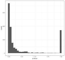
Multiple testing: Increase False Positive Rate
Multiple testing: Increase False Negative Risk
- Understand that we’re talking about a discovery process, not confirmation/validation.
- Strict (FWER) or less (FDR) control of Type I error does bad things for statistical power
- It actually hurts the discovery process!
Using standard multiple testing will typically only find the big hitters, which will probably have already been found
Taking names and giving prizes
- We often have the task of forwarding a promising biomarker from an (often large) set of candidates. So who gets the prize?
- This depends on the pool of candidates, the precision (or noise) of the response measurement, and the size of the training data
- If your training data is not big enough to help properly evaluate and “model out” the noise in the data, you’re not going to be very confident giving out prizes.
- If your response evaluation doesn’t provide strong enough signal, you’re not going to be very confident giving out prizes
- Prize-giving is what is called a “ranking and selection” problem, so it depends on the relative rather than absolute merits of the candidate biomarkers
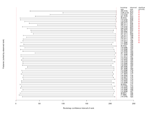
Biomarker selection using p-values is a ranking and selection problem
How can you evaluate your confidence in the prize winners?
- Resampling is your best friend here
- In particular, as a first pass, bootstrapping
- Repeat your full model-building and evaluation process on each bootstrap sample
- Figure out in each case which candidate gets which prize (gold, silver, bronze, platinum, copper, coal)
- Now see how often each candidate gets each prize (in other words, how often does a candidate get a particular rank)
- If a candidate consistently ranks high, cool.
- We can find that several candidates rank equally well
- Often, with small(ish) training data, we find that most candidates are all over the place. We’re just not in a good enough situation to give out prizes
Issues with multiple testing in feature selection
Main Issues during feature selection:
- The selection of the multiple testing correction method should depend on the the way the results are going to be used or reported.
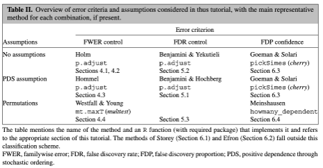
- Different methods control different things (see Table II). Discussion of this point is out of scope for this presentation.
- However, each choice has (bad) implications for statistical power, hence robustness of discovery
- Some popular correction methods assume gene expression independence!
- How many models were fitted in total? Was there a complete analysis plan made before collection?
- Regression to the mean (see next slide).
Good things always get worse (and bad things always improve)
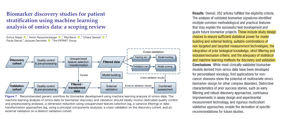
Developing a biomarker selection and validation pipeline
Three basic questions
What is a biomarker?
- A biological marker (biomarker) is a defined characteristic that is measured as an indicator of normal or pathogenic processes (prognosis), or biological response to an exposure or intervention (predictive).
What are biomarkers used for?
How do we develop a biomarker?
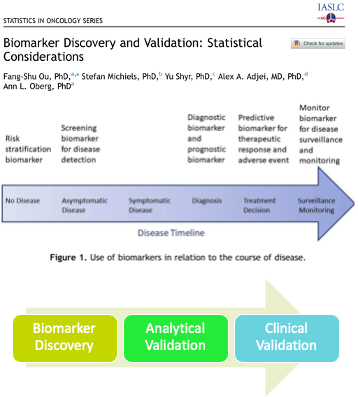
- 3 Phases: biomarker discovery, analytical validation and clinical validation.
- We will focus on the biomarker discovery phase.
What is the state of the art in biomarker discovery?
Recommendations
How best to make the initial feature reduction: from thousands to a few tens!
- Utilize any available biological insights or previous data – before starting!
- Bayesian approaches
- Knowledge graphs
- Reduce dimensionality of the problem and candidate correlations as much as possible
- Clustering, network centrality, etc
- Multivariate methods (regularized regression, etc)
- Utilize any available biological insights or previous data – before starting!
Test robustness and relevance
- Bootstrap or cross-validate
- Compare with the random-outcome dataset
- Use medically-relevant metrics
Curing dichotomania
Getting to good biomarkers: validity of what we discover
Prognostic biomarker indicates an increased (or decreased) likelihood of a future clinical event, disease recurrence or progression in an identified population
Considerations for the discovery of biological (molecular) targets
- quantifiable effect on risk over and above known clinical risk factors – how can we quantify this?
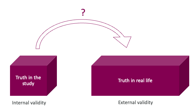
- internal and external validity – how can we check if the truth in the study is also the truth in real life?
- discover efficiently using limited data resources – what methods (e.g. stats) can be applied to the data that I have in hand?
Dichotomania
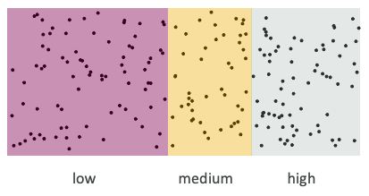
Taking information that exists on a continuous scale (such as blood pressure, lactate level, troponin) and transforming it into a binary or discrete cutoffs (e.g., “normal/abnormal”, “class 1/2/3”) for statistical and clinical convenience (Matt Sluba, 2021-02-28, link)
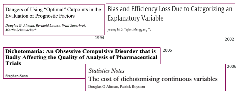
Statisticians have been highlighting this for decades
Natura non facit saltus
(Nature does not make jumps)
Gottfired Wilhelm Leibniz
Dichotomization and categorization (binning) of continuous data is still rampant. Especially in the prognostic/predictive biomarker space
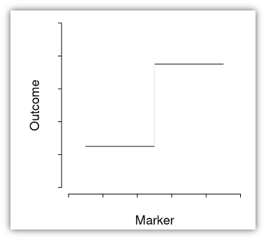
Dichotomization forces strong assumptions
This is (very very rarely) how Nature operates
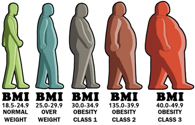
Implications of using BMI thresholds in models
- Suppose you are using BMI as a biomarker, and you dichotomize at 25 (the usual threshold for “normal”).
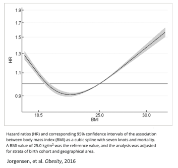
- You are saying that a person with a BMI of 24 is different from a person with a BMI of 26 and that this last person (with a BMI of 26) is no different from a person with a BMI of 40 – you are assuming persons with BMI of 26 or 40 share the same risk profile!
- To get around this, you may want to make many many cutoffs. If you make this decision, may as well treat things as continuous.
Real biomarkers are (often) hard to categorize
Statistical issues
Dichotomania results in poorer statistical properties and lowers efficiency
How well can the study results be generalized?
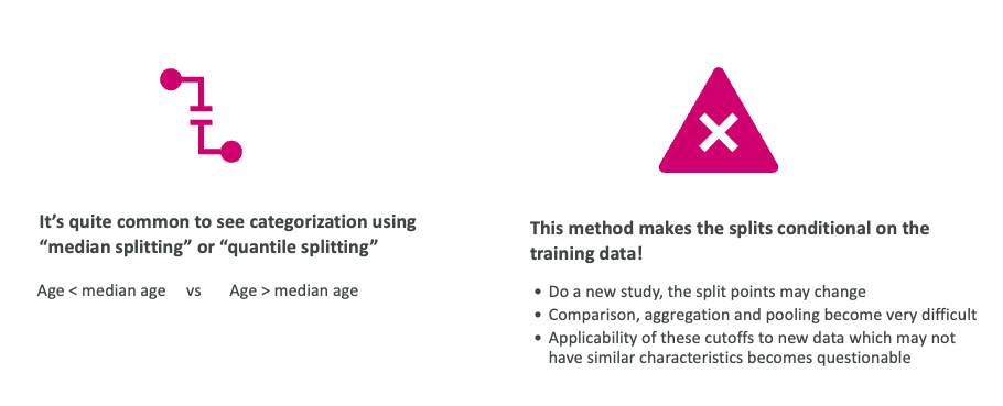
Taking medians or quantiles is not transferable
Statistical measures can’t find generalizable cutoffs
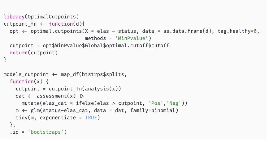
A common method of finding “optimal” cutoffs is the so-called “minimum p-value method (MinPVal)”
It take several candidate cutoff values and see which one provides the “most significant” difference in risk between the two sides, in terms of the smallest p-value.
Information is scarce and expensive: use it wisely
Dichotomization needs more data to make the same level of statistical inference compared to a continuous predictor
One interaction (for a predictive biomarker, for example) will need at least 4 times more data for a dichotomized prognostic biomarker compared to a continuous biomarker.
Linearity also results in information loss -> inefficiency -> misleading conclusions.
But probably it is not as bad as dichotomization.
Put patients first: do regression properly
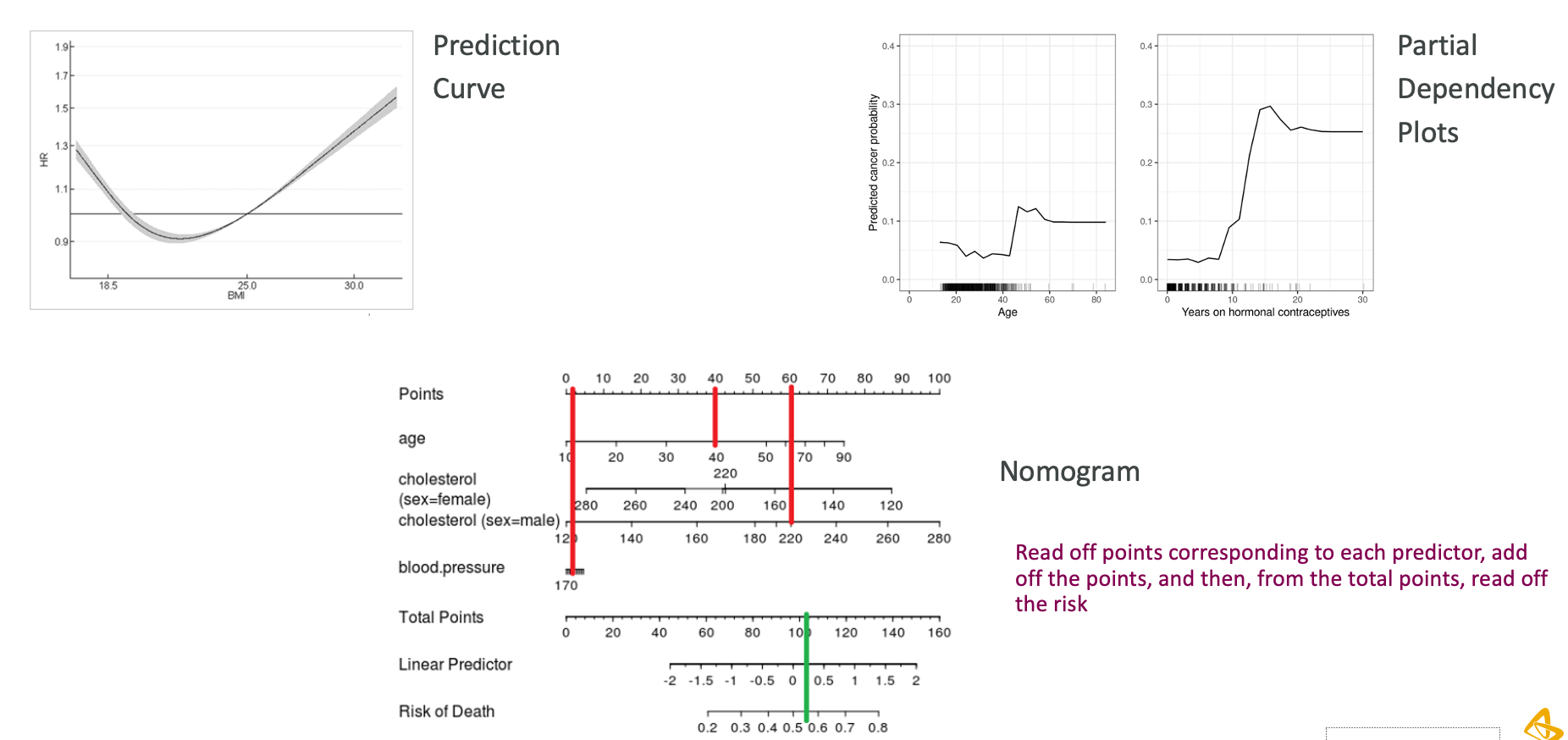
Use regression-based approaches to model the risk
These allow us to:
- Estimate the incremental improvement in risk prediction when adding a biomarker
- Either by explaining the risk variation or by predicting performance
- Control for overfitting through cross-validation and other means*
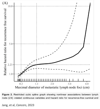
- To flexibly utilize the continuous nature of a continuous biomarker*
- Incorporate interactions and account for confounders that may affect a biomarker’s putative impact*
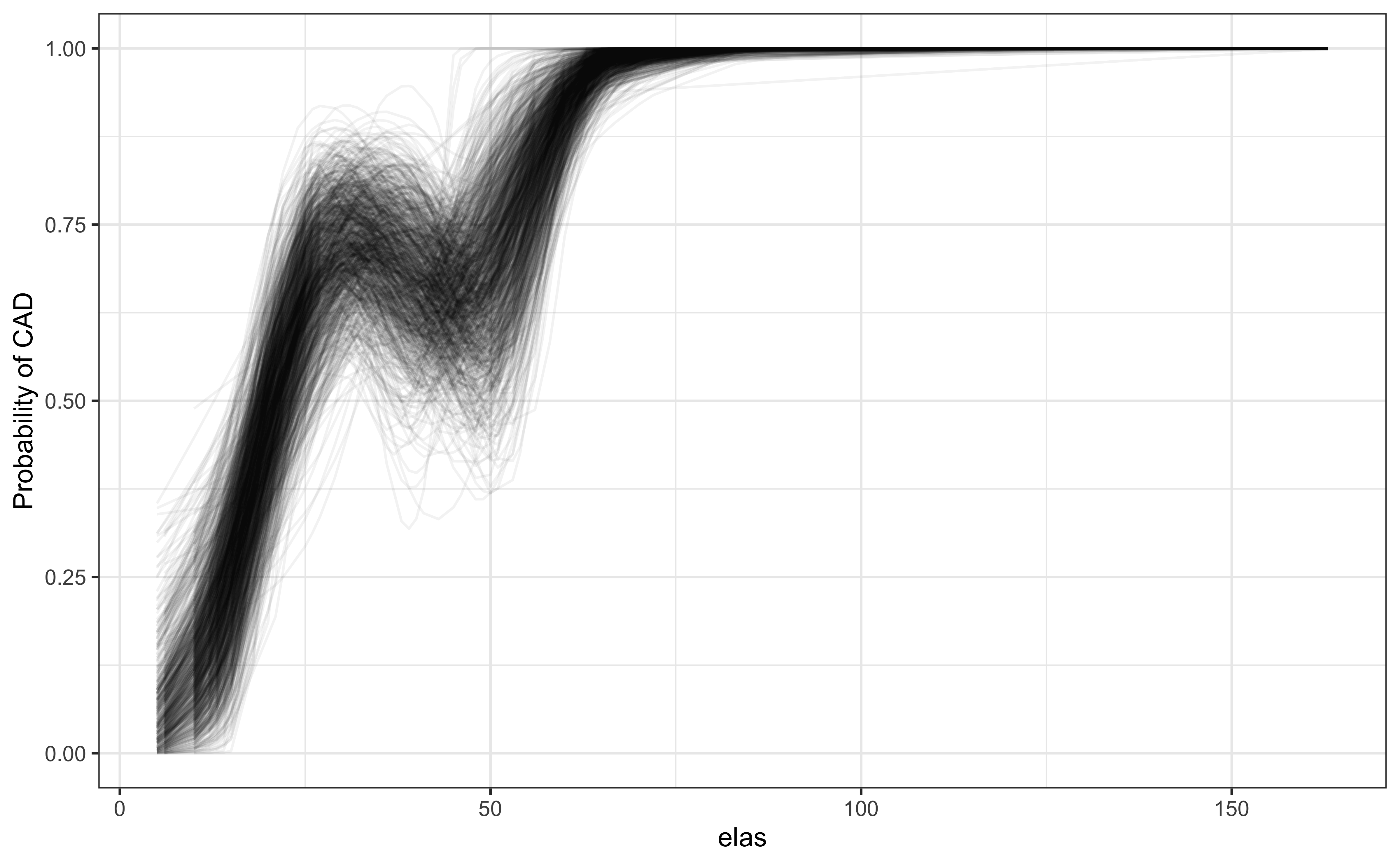
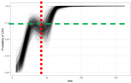
Bootstrapping shows consistency of the continuous relationship
P-value for elas (leukocyte elastase) is \(1.8\times 10^{-7}\)
set.seed(2048)
library(rsample)
btstrps <- bootstraps(elas, times = 1000)
models <- map_df(btstrps$splits,
        \(x) augment(glm(status ~ rcs(elas), data = analysis(x), family=binomial),
                     newdata=assessment(x), type.predict='response'),
        .id = 'bootstraps')
ggplot(models, aes(elas, .fitted, groups = bootstraps))+
  geom_line(alpha = 0.05)+ theme_bw()+
  labs(y = "Probability of CAD")
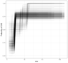
A computed threshold is quite variable and results in reduced statistical power and increased Type I error
Use continuous predictors!!
Start with known clinical risk factors
Add continuous biomarkers using flexible nonlinear constructs
- Spline functions
- Restricted cubic splines (rms::rcs in R)
- Splines in GAM models (mgcv::s in R)
- Fractional polynomials (mfp::fp in R)
- Spline functions
Simple statistics (likelihood ratio tests) assess whether the biomarker adds anything.
Resampling methods may help us understand the uncertainty and relevance of the biomarker, and help understand the degree of external validity we can expect
Ensure that we have good biomarkers
The observed effect of a biomarker may be partly obscured because of other risk factors (confounding)
- Proper study design, and incorporation of as many known factors as possible, helps with this.
- Accounting for potential confounders is important for generalization (e.g. concomitant medication, baseline status, CHIP effect, ….)
We may do better with multiple biomarkers as a panel rather than single biomarkers (BUT THIS IS HARDER)
- Interactions between biomarkers can be accounted for
- Still, don’t categorize but treat each continuous biomarker as continuous
Explanation and interpretation
“But Important People Don’t Understand This”
“But we need to decide based on the biomarker!”
- Dichotomization increases false negatives due to loss of statistical power.
- Eligibility criteria for entry into a clinical trial:
- We’ll miss eligible subjects!
- Eligibility for treatment:
- We’ll miss patients that could benefit from our treatments
- Eligibility criteria for entry into a clinical trial:
- Decide instead based on the continuous risk profile, not on arbitrary categories:
- The decision can be made on a threshold on the predicted risk from a model, which can result in threshold(s) on the biomarker values.
- If you need hard decisions, categorize at the very end, not at the beginning.
- Help decision-makers to understand their data!
Should we ever categorize?
- If you must, categorize in a data-independent way, before you look at the data.
- Categories may be based on business or medical decisions.
- For example, the categories for BMI are well-established and generally agreed upon.
- Categories may be based on business or medical decisions.
- Need to be careful that categories are only based on current knowledge
- Data leakage: predicting the future using the future!
Discrete (deterministic) thinking
This kind of discrete or deterministic thinking is not just a statistical manipulation, but often an way of thinking:
“discrete thinking is not simply something people do because they have to make decisions, nor is it something that people do just because they have some incentive to take a stance of certainty. So, when we’re talking about the problems of deterministic thinking, or premature collapse of the “wave function” of inferential uncertainty, we really are talking about a failure to incorporate enough of a continuous view of the world in our mental model.”
Andrew Gelman
DSAN 6150 | Fall 2024 | https://gu-dsan.github.io/6150-fall-2024
