Lecture 8

Spark Machine Learning

Amit Arora, Jeff Jacobs

Georgetown University

Fall 2025

Looking Back

Intro to Hadoop and MapReduce
Hadoop Streaming
Dask
Spark RDDs, DataFrames, SparkSQL

Future

Spark NLP
DataBricks on Azure
Spark Streaming

Today

Review of Distributed Hardware and Spark RDDs
Spark ML
Project Introduction
Lab:
- Practicing data cleaning with Spark DataFrames
- Using Spark ML
Quiz on Hadoop Streaming and HDFS (due Friday October 14)

Essential Prior Topics

AWS Academy

Credit limit - $100
Course numbers:
- Course #1 - 24178
- Course #2 - 27354
- Course #3 - 22802
- Course #4 - 26418

STAY WITH COURSE 24178 UNLESS YOU HAVE RUN OUT OF CREDITS OR >$90 USED!

Note that you will have to repeat several setup steps:

security group
EC2 keypair uploading (the AWS part only)
sagemaker setup
any S3 uploading or copying as well as bucket creation as necessary
EMR configuration

Grades

You are responsible for your grades
If there is a problem, you need to bring it up
All assignments are mandatory
State of assignments from syllabus
Group Project: 30%
HW Assignments: 45%
Lab Deliverables: 15% - Halfway through
Quizzes: 10% - One to two more

Review of File Systems

What are the possible file system options for each item: S3, HDFS, Local file system

hadoop jar /usr/lib/hadoop/hadoop-streaming.jar #1

-files basic-mapper.py,basic-reducer.py #2

-input /user/hadoop/in_data #3
-output /user/hadoop/in_data #3

-mapper basic-mapper.py #4
-reducer basic-reducer.py #4

Local file system

Local file system or S3

HDFS or S3

HDFS - why??

Spark: a Unified Engine

Connected and extensible

Caching and Persistence

By default, RDDs are recomputed every time you run an action on them. This can be expensive (in time) if you need to use a dataset more than once.

Spark allows you to control what is cached in memory.

To tell spark to cache an object in memory, use persist() or cache():

cache(): is a shortcut for using default storage level, which is memory only
persist(): can be customized to other ways to persist data (including both memory and/or disk)

# caches error RDD in memory, but only after an action is run
errors = logs.filter(lambda x: "error" in x and "2019-12" in x).cache()

Review of PySparkSQL Cheatsheet

https://s3.amazonaws.com/assets.datacamp.com/blog_assets/PySpark_SQL_Cheat_Sheet_Python.pdf

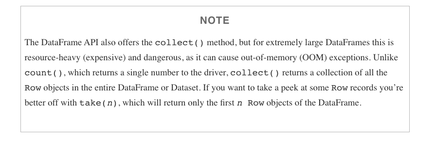
`collect` CAUTION

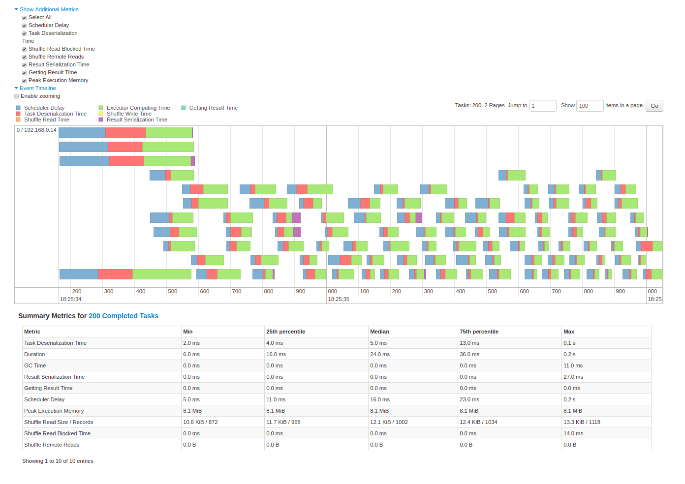
Spark Diagnostic UI

Understanding how the cluster is running your job

Spark Application UI shows important facts about you Spark job:

Event timeline for each stage of your work
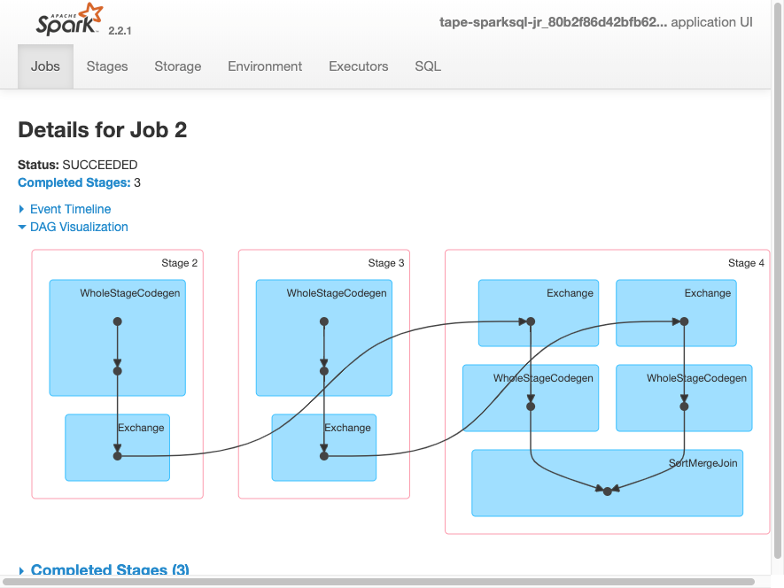
Directed acyclical graph (DAG) of your job
Spark job history
Status of Spark executors
Physical / logical plans for any SQL queries

Tool to confirm you are getting the horizontal scaling that you need!

Adapted from AWS Glue Spark UI docs and Spark UI docs

Spark UI - Event timeline

Spark UI - DAG

Spark UI - Job History

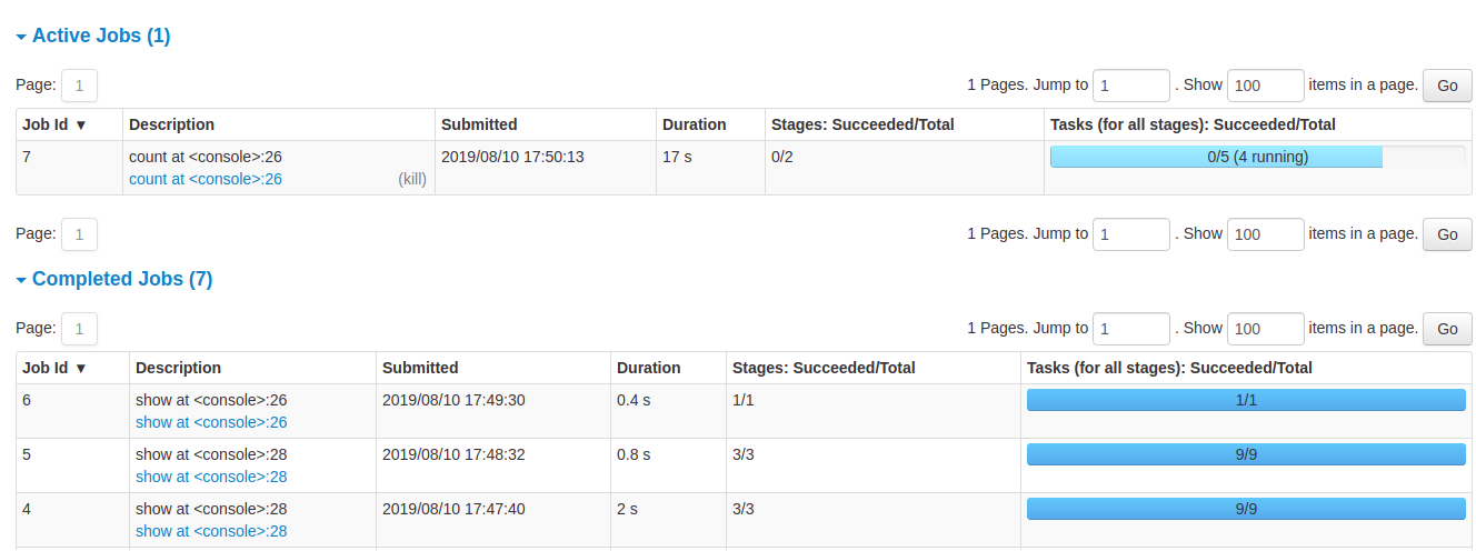
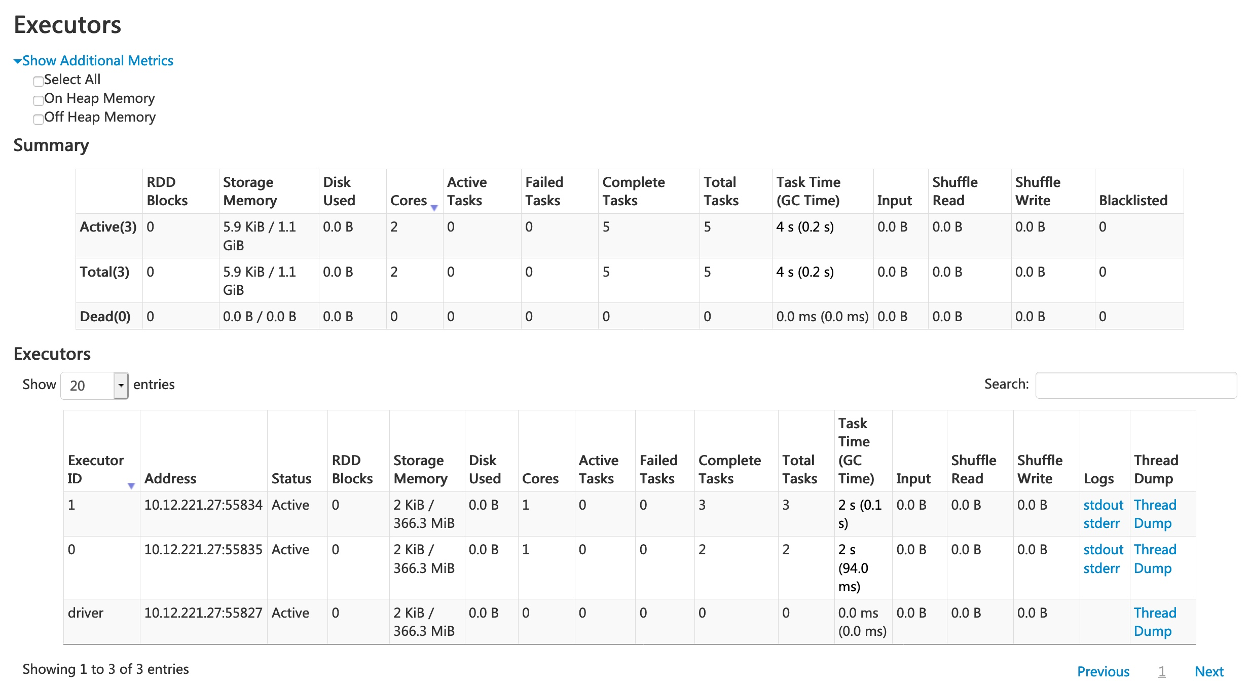
Spark UI - Executors

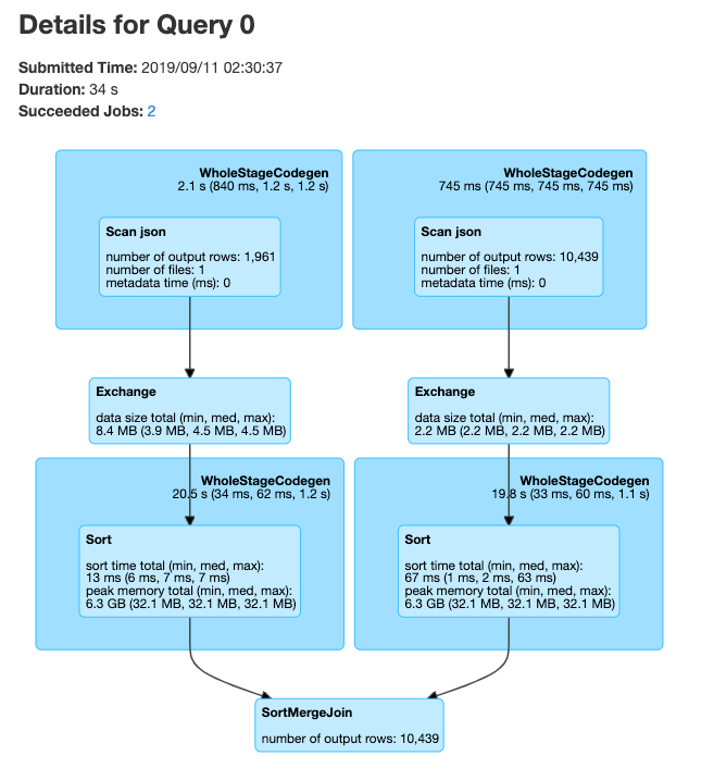
Spark UI - SQL

PySpark User Defined Functions

UDF Workflow

Adapted from UDFs in Spark

UDF Example

Problem: make a new column with ages for adults-only

+-------+--------------+
|room_id|   guests_ages|
+-------+--------------+
|      1|  [18, 19, 17]|
|      2|   [25, 27, 5]|
|      3|[34, 38, 8, 7]|
+-------+--------------+

UDF Code Solution

from pyspark.sql.functions import udf, col

@udf("array<integer>")
   def filter_adults(elements):
   return list(filter(lambda x: x >= 18, elements))

# alternatively
from pyspark.sql.types IntegerType, ArrayType
@udf(returnType=ArrayType(IntegerType()))
def filter_adults(elements):
   return list(filter(lambda x: x >= 18, elements))

+-------+----------------+------------+
|room_id| guests_ages    | adults_ages|
+-------+----------------+------------+
| 1     | [18, 19, 17]   |    [18, 19]|
| 2     | [25, 27, 5]    |    [25, 27]|
| 3     | [34, 38, 8, 7] |    [34, 38]|
| 4     |[56, 49, 18, 17]|[56, 49, 18]|
+-------+----------------+------------+

Alternative to Spark UDF

# Spark 3.1
from pyspark.sql.functions import col, filter, lit

df.withColumn('adults_ages',
              filter(col('guests_ages'), lambda x: x >= lit(18))).show()

UDF Speed Comparison

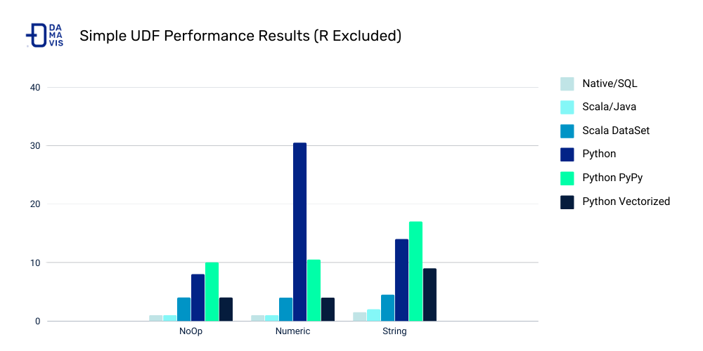
Costs:

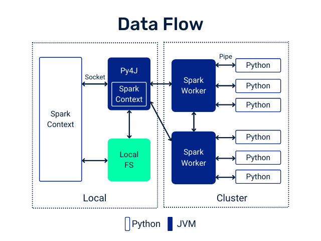
Serialization/deserialization (think pickle files)
Data movement between JVM and Python
Less Spark optimization possible

Other ways to make your Spark jobs faster source:

Cache/persist your data into memory
Using Spark DataFrames over Spark RDDs
Using Spark SQL functions before jumping into UDFs
Save to serialized data formats like Parquet

Pandas UDF

From PySpark docs - Pandas UDFs are user defined functions that are executed by Spark using Arrow to transfer data and Pandas to work with the data, which allows vectorized operations. A Pandas UDF is defined using the pandas_udf as a decorator or to wrap the function, and no additional configuration is required. A Pandas UDF behaves as a regular PySpark function API in general.

@pandas_udf("string")
def to_upper(s: pd.Series) -> pd.Series:
    return s.str.upper()

df = spark.createDataFrame([("John Doe",)], ("name",))
df.select(to_upper("name")).show()
+--------------+
|to_upper(name)|
+--------------+
|      JOHN DOE|
+--------------+

@pandas_udf("first string, last string")
def split_expand(s: pd.Series) -> pd.DataFrame:
    return s.str.split(expand=True)


df = spark.createDataFrame([("John Doe",)], ("name",))
df.select(split_expand("name")).show()
+------------------+
|split_expand(name)|
+------------------+
|       [John, Doe]|
+------------------+

https://spark.apache.org/docs/3.1.2/api/python/reference/api/pyspark.sql.functions.pandas_udf.html

Assumption: knowledge of ML techniques and process

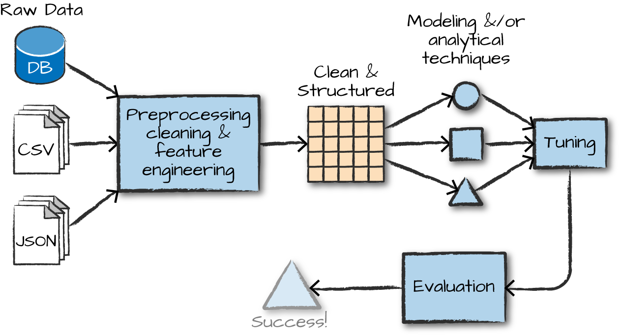
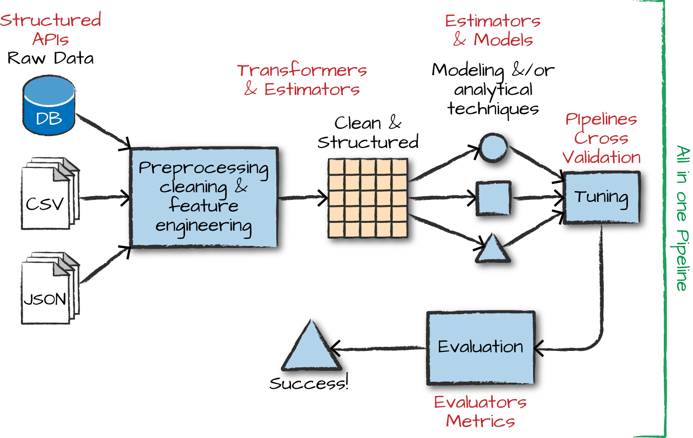
Overview of ML

The advanced analytics/ML process

Gather and collect data
Clean and inspect data
Perform feature engineering
Split data into train/test
Evaluate and compare models

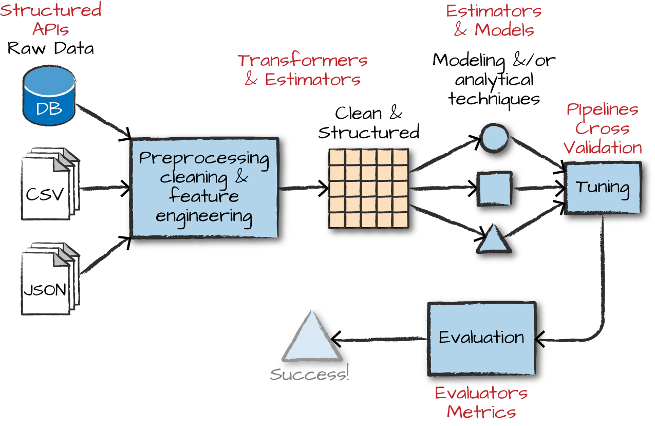
ML with Spark

What is `MLlib`

Capabilities

Gather and clean data
Perform feature engineering
Perform feature selection
Train and tune models
Put models in production

API is divided into two packages

org.apache.spark.ml (High level API) - Provides higher level API built on top of DataFrames - Allows the construction of ML pipelines

org.apache.spark.mllib (Predates DataFrames) - Original API built on top of RDDs

Inspired by `scikit-learn`

DataFrame
Transformer
Estimator
Pipeline
Parameter

Transformers, esimators, and pipelines

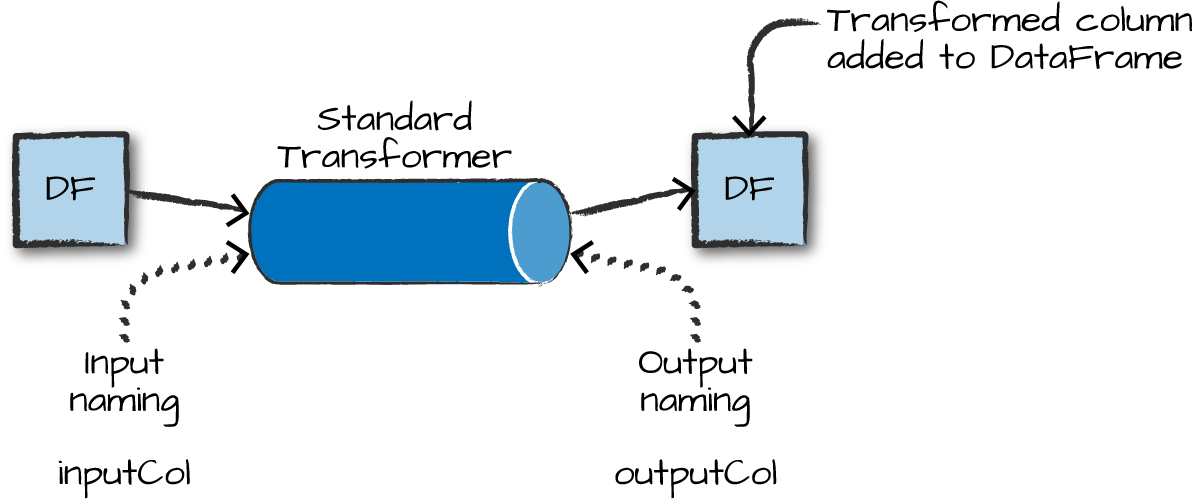
Transformers

Transformers take DataFrames as input, and return a new DataFrame as output. Transformers do not learn any parameters from the data, they simply apply rule-based transformations to either prepare data for model training or generate predictions using a trained model.

Transformers are run using the .transform() method

Some Examples of Transformers

Converting categorical variables to numeric (must do this)
- StringIndexer
- OneHotEncoder can act on multiple columns at a time
Data Normalization
- Normalizer
- StandardScaler
String Operations
- Tokenizer
- StopWordsRemover
- PCA
Converting continuous to discrete
- Bucketizer
- QuantileDiscretizer
Many more
- Spark 2.4.7: http://spark.apache.org/docs/2.4.7/ml-guide.html
- Spark 3.1.1: http://spark.apache.org/docs/3.1.1/ml-guide.html

`MLlib` algorithms for machine learning models need single, numeric features column as input

Each row in this column contains a vector of data points corresponding to the set of features used for prediction.

Use the VectorAssembler transformer to create a single vector column from a list of columns.
All categorical data needs to be numeric for machine learning

# Example from Spark docs
from pyspark.ml.linalg import Vectors
from pyspark.ml.feature import VectorAssembler

dataset = spark.createDataFrame(
    [(0, 18, 1.0, Vectors.dense([0.0, 10.0, 0.5]), 1.0)],
    ["id", "hour", "mobile", "userFeatures", "clicked"])

assembler = VectorAssembler(
    inputCols=["hour", "mobile", "userFeatures"],
    outputCol="features")

output = assembler.transform(dataset)
print("Assembled columns 'hour', 'mobile', 'userFeatures' to vector column 'features'")
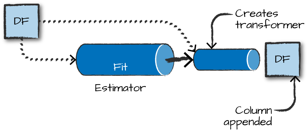
output.select("features", "clicked").show(truncate=False)

Estimators

Estimators learn (or “fit”) parameters from your DataFrame via the .fit() method, and return a model which is a Transformer

Pipelines

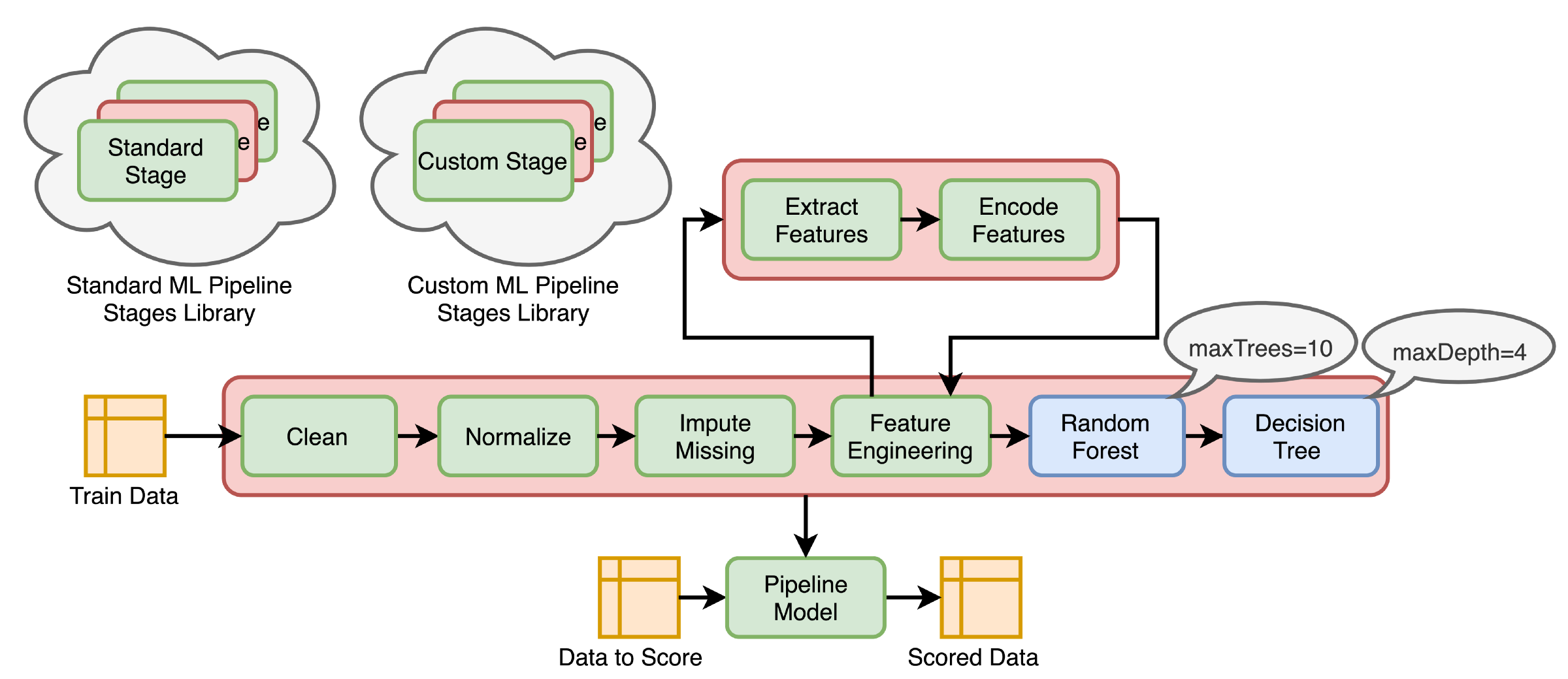
Pipelines combine multiple steps into a single workflow that can be easily run. * Data cleaning and feature processing via transformers, using stages * Model definition * Run the pipeline to do all transformations and fit the model

The Pipeline constructor takes an array of pipeline stages

Why Pipelines?

Cleaner Code: Accounting for data at each step of preprocessing can get messy. With a Pipeline, you won’t need to manually keep track of your training and validation data at each step.
Fewer Bugs: There are fewer opportunities to misapply a step or forget a preprocessing step.
Easier to Productionize: It can be surprisingly hard to transition a model from a prototype to something deployable at scale, but Pipelines can help.
More Options for Model Validation: We can easily apply cross-validation and other techniques to our Pipelines.

Example

Using the HMP Dataset. The structure of the dataset looks like this:

# read data from text file and split each line into words
df.printSchema()

root  
|-- x: integer (nullable = true)  
|-- y: integer (nullable = true)  
|-- z: integer (nullable = true)  
|-- class: string (nullable = false)  
|-- source: string (nullable = false)

Let’s transform strings to numbers

The StringIndexer is an estimator having both fit and transform methods.
To create a StringIndexer object (indexer), pass the class column as inputCol, and classIndex as outputCol.
Then we fit the DataFrame to the indexer (to run the estimator), and transform the DataFrame. This creates a brand new DataFrame (indexed), which we can see below, containing the classIndex additional column.

from pyspark.ml.feature import StringIndexer

indexer = StringIndexer(inputCol = 'class', outputCol = 'classIndex')
indexed = indexer.fit(df).transform(df)  # This is a new data frame

# Let's see it
indexed.show(5)

+---+---+---+-----------+--------------------+----------+
|  x|  y|  z|      class|              source|classIndex|
+---+---+---+-----------+--------------------+----------+
| 29| 39| 51|Drink_glass|Accelerometer-201...|       2.0|
| 29| 39| 51|Drink_glass|Accelerometer-201...|       2.0|
| 28| 38| 52|Drink_glass|Accelerometer-201...|       2.0|
| 29| 37| 51|Drink_glass|Accelerometer-201...|       2.0|
| 30| 38| 52|Drink_glass|Accelerometer-201...|       2.0|
+---+---+---+-----------+--------------------+----------+
only showing top 5 rows

One-Hot Encode categorical variables

Unlike the StringIndexer, OneHotEncoder is a pure transformer, having only the transform method. It uses the same syntax of inputCol and outputCol.
OneHotEncoder creates a brand new DataFrame (encoded), with a category_vec column added to the previous DataFrame(indexed).
OneHotEncoder doesn’t return several columns containing only zeros and ones; it returns a sparse-vector as seen in the categoryVec column. Thus, for the ‘Drink_glass’ class above, SparkML returns a sparse-vector that basically says there are 13 elements, and at position 2, the class value exists(1.0).

from pyspark.ml.feature import OneHotEncoder

# The OneHotEncoder is a pure transformer object. it does not use the fit()
encoder = OneHotEncoder(inputCol = 'classIndex', outputCol = 'categoryVec')
encoded = encoder.transform(indexed)  # This is a new data frame
encoded.show(5, False)

+---+---+---+-----------+----------------------------------------------------+----------+--------------+
|x  |y  |z  |class      |source                                              |classIndex|categoryVec   |
+---+---+---+-----------+----------------------------------------------------+----------+--------------+
|29 |39 |51 |Drink_glass|Accelerometer-2011-06-01-14-13-57-drink_glass-f1.txt|2.0       |(13,[2],[1.0])|
|29 |39 |51 |Drink_glass|Accelerometer-2011-06-01-14-13-57-drink_glass-f1.txt|2.0       |(13,[2],[1.0])|
|28 |38 |52 |Drink_glass|Accelerometer-2011-06-01-14-13-57-drink_glass-f1.txt|2.0       |(13,[2],[1.0])|
|29 |37 |51 |Drink_glass|Accelerometer-2011-06-01-14-13-57-drink_glass-f1.txt|2.0       |(13,[2],[1.0])|
|30 |38 |52 |Drink_glass|Accelerometer-2011-06-01-14-13-57-drink_glass-f1.txt|2.0       |(13,[2],[1.0])|
+---+---+---+-----------+----------------------------------------------------+----------+--------------+
only showing top 5 rows

Assembling the feature vector

The VectorAssembler object gets initialized with the same syntax as StringIndexer and OneHotEncoder.
The list ['x', 'y', 'z'] is paseed to inputCols, and we specify outputCol = ‘features’.
This is also a pure transformer.

from pyspark.ml.linalg import Vectors
from pyspark.ml.feature import VectorAssembler
# VectorAssembler creates vectors from ordinary data types for us

vectorAssembler = VectorAssembler(inputCols = ['x','y','z'], outputCol = 'features')
# Now we use the vectorAssembler object to transform our last updated dataframe

features_vectorized = vectorAssembler.transform(encoded)  # note this is a new df

features_vectorized.show(5, False)

+---+---+---+-----------+----------------------------------------------------+----------+--------------+----------------+
|x  |y  |z  |class      |source                                              |classIndex|categoryVec   |features        |
+---+---+---+-----------+----------------------------------------------------+----------+--------------+----------------+
|29 |39 |51 |Drink_glass|Accelerometer-2011-06-01-14-13-57-drink_glass-f1.txt|2.0       |(13,[2],[1.0])|[29.0,39.0,51.0]|
|29 |39 |51 |Drink_glass|Accelerometer-2011-06-01-14-13-57-drink_glass-f1.txt|2.0       |(13,[2],[1.0])|[29.0,39.0,51.0]|
|28 |38 |52 |Drink_glass|Accelerometer-2011-06-01-14-13-57-drink_glass-f1.txt|2.0       |(13,[2],[1.0])|[28.0,38.0,52.0]|
|29 |37 |51 |Drink_glass|Accelerometer-2011-06-01-14-13-57-drink_glass-f1.txt|2.0       |(13,[2],[1.0])|[29.0,37.0,51.0]|
|30 |38 |52 |Drink_glass|Accelerometer-2011-06-01-14-13-57-drink_glass-f1.txt|2.0       |(13,[2],[1.0])|[30.0,38.0,52.0]|
+---+---+---+-----------+----------------------------------------------------+----------+--------------+----------------+
only showing top 5 rows

Normalizing the dataset

Normalizer like all transformers have consistent syntax. Looking at the Normalizer object, it contains the parameter p=1.0 (the default norm value for Pyspark Normalizer is p=2.0.)
p=1.0 uses Manhattan Distance
p=2.0 uses Euclidean Distance

from pyspark.ml.feature import Normalizer
normalizer = Normalizer(inputCol = 'features', outputCol = 'features_norm', p=1.0)  # Manhattan Distance
normalized_data = normalizer.transform(features_vectorized) # New data frame too.

normalized_data.show(5)
>>
+---+---+---+-----------+--------------------+----------+--------------+----------------+--------------------+
|  x|  y|  z|      class|              source|classIndex|   categoryVec|        features|       features_norm|
+---+---+---+-----------+--------------------+----------+--------------+----------------+--------------------+
| 29| 39| 51|Drink_glass|Accelerometer-201...|       2.0|(13,[2],[1.0])|[29.0,39.0,51.0]|[0.24369747899159...|
| 29| 39| 51|Drink_glass|Accelerometer-201...|       2.0|(13,[2],[1.0])|[29.0,39.0,51.0]|[0.24369747899159...|
| 28| 38| 52|Drink_glass|Accelerometer-201...|       2.0|(13,[2],[1.0])|[28.0,38.0,52.0]|[0.23728813559322...|
| 29| 37| 51|Drink_glass|Accelerometer-201...|       2.0|(13,[2],[1.0])|[29.0,37.0,51.0]|[0.24786324786324...|
| 30| 38| 52|Drink_glass|Accelerometer-201...|       2.0|(13,[2],[1.0])|[30.0,38.0,52.0]|[0.25,0.316666666...|
+---+---+---+-----------+--------------------+----------+--------------+----------------+--------------------+
only showing top 5 rows

Running the transformation `Pipeline`

The Pipeline constructor below takes an array of Pipeline stages we pass to it. Here we pass the 4 stages defined earlier, in the right sequence, one after another.

from pyspark.ml import Pipeline
pipeline = Pipeline(stages = [indexer,encoder,vectorAssembler,normalizer])

Now the Pipeline object fit to our original DataFrame df

data_model = pipeline.fit(df)

Finally, we transform our DataFrame df using the Pipeline Object.

pipelined_data = data_model.transform(df)

pipelined_data.show(5)

+---+---+---+-----------+--------------------+----------+--------------+----------------+--------------------+
|  x|  y|  z|      class|              source|classIndex|   categoryVec|        features|       features_norm|
+---+---+---+-----------+--------------------+----------+--------------+----------------+--------------------+
| 29| 39| 51|Drink_glass|Accelerometer-201...|       2.0|(13,[2],[1.0])|[29.0,39.0,51.0]|[0.24369747899159...|
| 29| 39| 51|Drink_glass|Accelerometer-201...|       2.0|(13,[2],[1.0])|[29.0,39.0,51.0]|[0.24369747899159...|
| 28| 38| 52|Drink_glass|Accelerometer-201...|       2.0|(13,[2],[1.0])|[28.0,38.0,52.0]|[0.23728813559322...|
| 29| 37| 51|Drink_glass|Accelerometer-201...|       2.0|(13,[2],[1.0])|[29.0,37.0,51.0]|[0.24786324786324...|
| 30| 38| 52|Drink_glass|Accelerometer-201...|       2.0|(13,[2],[1.0])|[30.0,38.0,52.0]|[0.25,0.316666666...|
+---+---+---+-----------+--------------------+----------+--------------+----------------+--------------------+
only showing top 5 rows

One last step before training

# first let's list out the columns we want to drop
cols_to_drop = ['x','y','z','class','source','classIndex','features']

# Next let's use a list comprehension with conditionals to select cols we need
selected_cols = [col for col in pipelined_data.columns if col not in cols_to_drop]

# Let's define a new train_df with only the categoryVec and features_norm cols
df_train = pipelined_data.select(selected_cols)

# Let's see our training dataframe.
df_train.show(5)

+--------------+--------------------+
|   categoryVec|       features_norm|
+--------------+--------------------+
|(13,[2],[1.0])|[0.24369747899159...|
|(13,[2],[1.0])|[0.24369747899159...|
|(13,[2],[1.0])|[0.23728813559322...|
|(13,[2],[1.0])|[0.24786324786324...|
|(13,[2],[1.0])|[0.25,0.316666666...|
only showing top 5 rows

You now have a DataFrame optimized for SparkML!

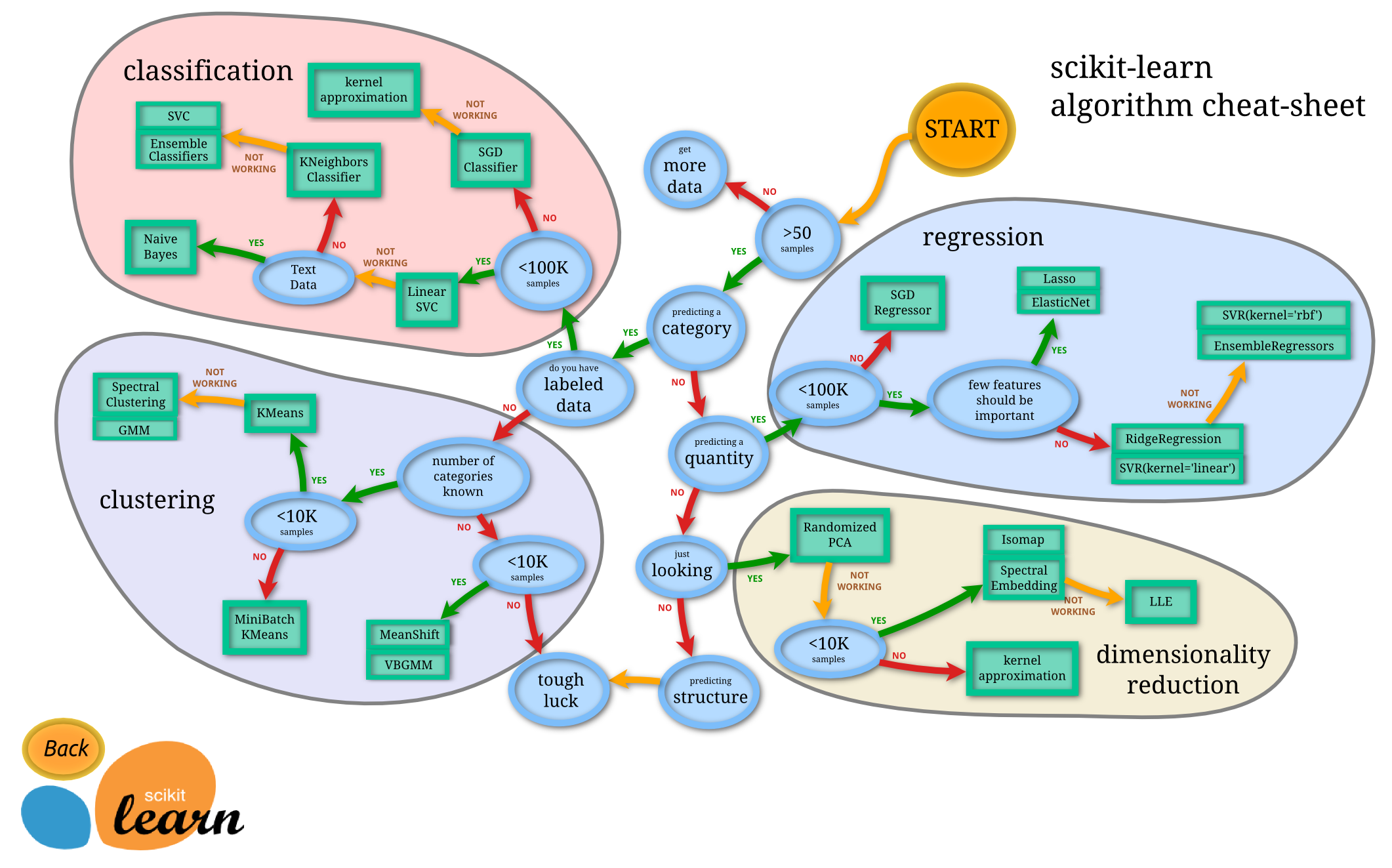
Machine Learning Models in Spark

There are many Spark machine learning models

Regression

Linear regression - what is the optimization method?
Survival regression
Genearlized linear model (GLM)
Random forest regression

Classification

Logistic regression
Gradient-boosted tree model (GBM)
Naive Bayes
Multilayer perception (neural network!)

Other

Clustering (K-means, LDA, GMM)
Association rule mining

Building your Model

Feature selection using easy R-like formulas

# Example from Spark docs
from pyspark.ml.feature import RFormula

dataset = spark.createDataFrame(
    [(7, "US", 18, 1.0),
     (8, "CA", 12, 0.0),
     (9, "NZ", 15, 0.0)],
    ["id", "country", "hour", "clicked"])

formula = RFormula(
    formula="clicked ~ country + hour",
    featuresCol="features",
    labelCol="label")

output = formula.fit(dataset).transform(dataset)
output.select("features", "label").show()

What if you have too many columns for your model?

Evaluating 1,000s or 10,000s of variables?

Chi-Squared Selector

Pick categorical variables that are most dependent on the response variable

Can even check the p-values of specific variables!

# Example from Spark docs
from pyspark.ml.feature import ChiSqSelector
from pyspark.ml.linalg import Vectors

df = spark.createDataFrame([
    (7, Vectors.dense([0.0, 0.0, 18.0, 1.0]), 1.0,),
    (8, Vectors.dense([0.0, 1.0, 12.0, 0.0]), 0.0,),
    (9, Vectors.dense([1.0, 0.0, 15.0, 0.1]), 0.0,)], ["id", "features", "clicked"])

selector = ChiSqSelector(numTopFeatures=1, featuresCol="features",
                         outputCol="selectedFeatures", labelCol="clicked")

result = selector.fit(df).transform(df)

print("ChiSqSelector output with top %d features selected" % selector.getNumTopFeatures())
result.show()

Tuning your model

Part 1

# Example from Spark docs
from pyspark.ml.evaluation import RegressionEvaluator
from pyspark.ml.regression import LinearRegression
from pyspark.ml.tuning import ParamGridBuilder, TrainValidationSplit

# Prepare training and test data.
data = spark.read.format("libsvm")\
    .load("data/mllib/sample_linear_regression_data.txt")
train, test = data.randomSplit([0.9, 0.1], seed=12345)

lr = LinearRegression(maxIter=10)

# We use a ParamGridBuilder to construct a grid of parameters to search over.
# TrainValidationSplit will try all combinations of values and determine best model using
# the evaluator.
paramGrid = ParamGridBuilder()\
    .addGrid(lr.regParam, [0.1, 0.01]) \
    .addGrid(lr.fitIntercept, [False, True])\
    .addGrid(lr.elasticNetParam, [0.0, 0.5, 1.0])\
    .build()

Tuning your model

Part 2

# In this case the estimator is simply the linear regression.
# A TrainValidationSplit requires an Estimator, a set of Estimator ParamMaps, and an Evaluator.
tvs = TrainValidationSplit(estimator=lr,
                           estimatorParamMaps=paramGrid,
                           evaluator=RegressionEvaluator(),
                           # 80% of the data will be used for training, 20% for validation.
                           trainRatio=0.8)

# Run TrainValidationSplit, and choose the best set of parameters.
model = tvs.fit(train)

# Make predictions on test data. model is the model with combination of parameters
# that performed best.
model.transform(test)\
    .select("features", "label", "prediction")\
    .show()

Lecture 8

Looking Back

Future

Today

Essential Prior Topics

AWS Academy

Grades

Review of File Systems

Spark: a Unified Engine

Connected and extensible

Caching and Persistence

Review of PySparkSQL Cheatsheet

collect CAUTION

Spark Diagnostic UI

Understanding how the cluster is running your job

Tool to confirm you are getting the horizontal scaling that you need!

Spark UI - Event timeline

Spark UI - DAG

Spark UI - Job History

Spark UI - Executors

Spark UI - SQL

PySpark User Defined Functions

UDF Workflow

UDF Example

UDF Code Solution

Alternative to Spark UDF

UDF Speed Comparison

Pandas UDF

Assumption: knowledge of ML techniques and process

Overview of ML

The advanced analytics/ML process

ML with Spark

What is MLlib

Capabilities

API is divided into two packages

Inspired by scikit-learn

Transformers, esimators, and pipelines

Transformers

Some Examples of Transformers

MLlib algorithms for machine learning models need single, numeric features column as input

Estimators

Pipelines

Pipelines

Why Pipelines?

Example

Let’s transform strings to numbers

One-Hot Encode categorical variables

Assembling the feature vector

Normalizing the dataset

Running the transformation Pipeline

One last step before training

You now have a DataFrame optimized for SparkML!

Machine Learning Models in Spark

Regression

Classification

Other

Building your Model

What if you have too many columns for your model?

Chi-Squared Selector

Tuning your model

Part 1

Tuning your model

Part 2

Lab

`collect` CAUTION

What is `MLlib`

Inspired by `scikit-learn`

`MLlib` algorithms for machine learning models need single, numeric features column as input

Running the transformation `Pipeline`