Lecture 9

SparkML

Amit Arora, Abhijit Dasgupta, Anderson Monken, and Marck Vaisman

Georgetown University

Fall 2023

Logistics and Review

Deadlines

Lab 7: Spark DataFrames Due Oct 10 6pm
Lab 8: SparkNLP Due Oct 17 6pm
Assignment 6: Spark (Multi-part) Due Oct 23 11:59pm
Lab 9: SparkML Due Oct 24 6pm
Lab 10: Spark Streaming Due Oct 31 6pm
Lab 11: Dask Due Nov 7 6pm
Lab 12: Ray Due Nov 14 6pm

Look back and ahead

Searching Slack for existing Q&A - like StackOverflow!
Spark RDDs, Spark DataFrames, Spark UDFs
Now: SparkML and project
Next week: Spark Streaming

Review of Prior Topics

AWS Academy

Credit limit - $100
Course numbers:
- Course #1 - 54380
- Course #2 - 54378

STAY WITH COURSE 54380 UNLESS YOU HAVE RUN OUT OF CREDITS OR >$90 USED!

Note that you will have to repeat several setup steps:

SageMaker domain set up (review Slack channel to review solutiosn to issues)
any S3 uploading or copying as well as bucket creation as necessary

Caching and Persistence

By default, RDDs are recomputed every time you run an action on them. This can be expensive (in time) if you need to use a dataset more than once.

Spark allows you to control what is cached in memory.

To tell spark to cache an object in memory, use persist() or cache():

cache(): is a shortcut for using default storage level, which is memory only
persist(): can be customized to other ways to persist data (including both memory and/or disk)

# caches error RDD in memory, but only after an action is run
errors = logs.filter(lambda x: "error" in x and "2019-12" in x).cache()

`collect` CAUTION

Assumption: knowledge of ML techniques and process

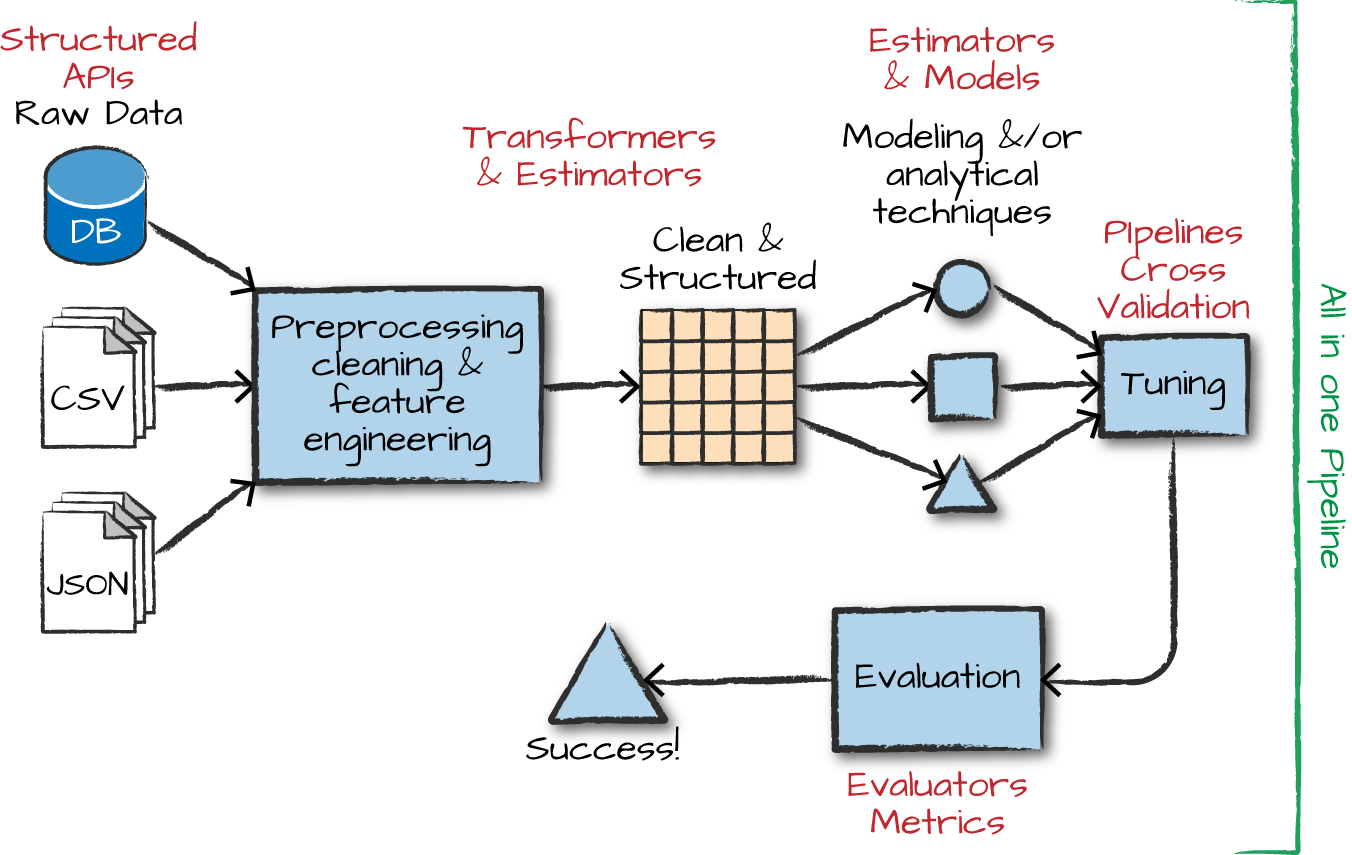
Overview of ML

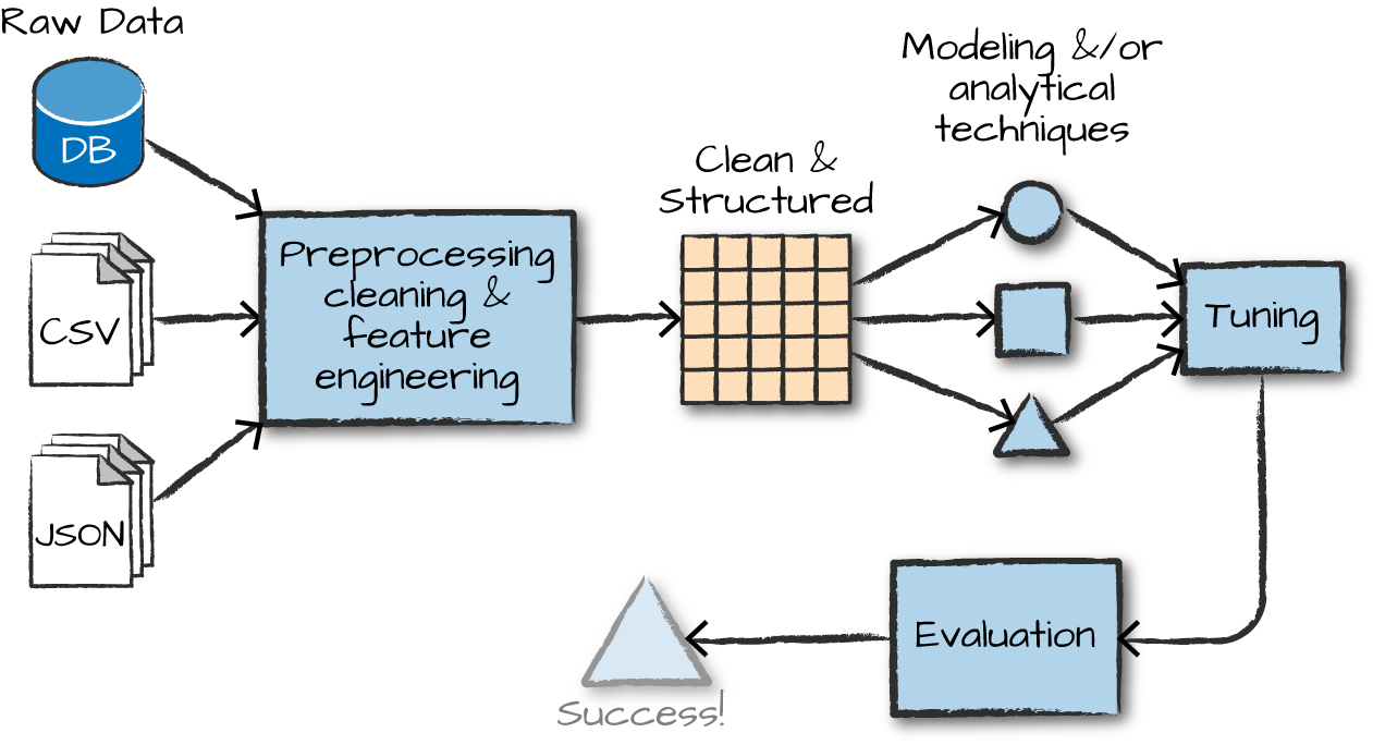
The advanced analytics/ML process

Gather and collect data
Clean and inspect data
Perform feature engineering
Split data into train/test
Evaluate and compare models

ML with Spark

What is `MLlib`

Capabilities

Gather and clean data
Perform feature engineering
Perform feature selection
Train and tune models
Put models in production

API is divided into two packages

org.apache.spark.ml (High-level API) - Provides higher level API built on top of DataFrames - Allows the construction of ML pipelines

org.apache.spark.mllib (Predates DataFrames - in maintenance mode) - Original API built on top of RDDs

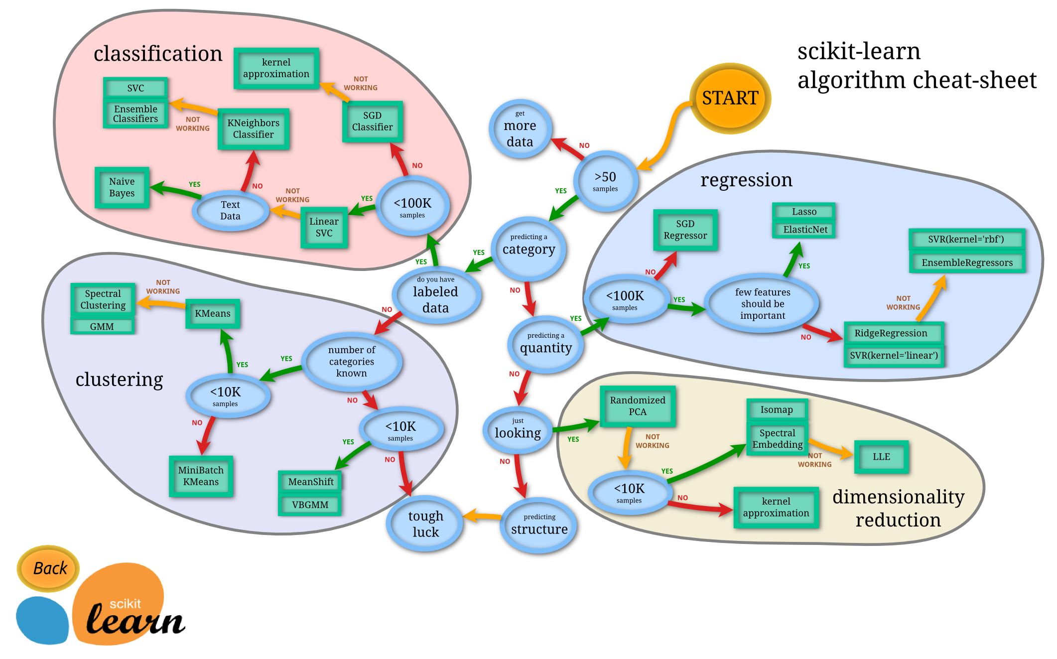
Inspired by `scikit-learn`

DataFrame
Transformer
Estimator
Pipeline
Parameter

Transformers, estimators, and pipelines

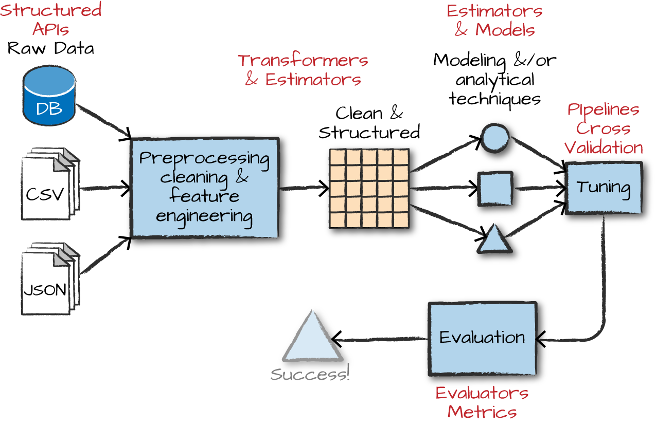
Transformers

Transformers takes DataFrames as input, and return a new DataFrame as output. Transformers do not learn any parameters from the data, they simply apply rule-based transformations to either prepare data for model training or generate predictions using a trained model.

Transformers are run using the .transform() method

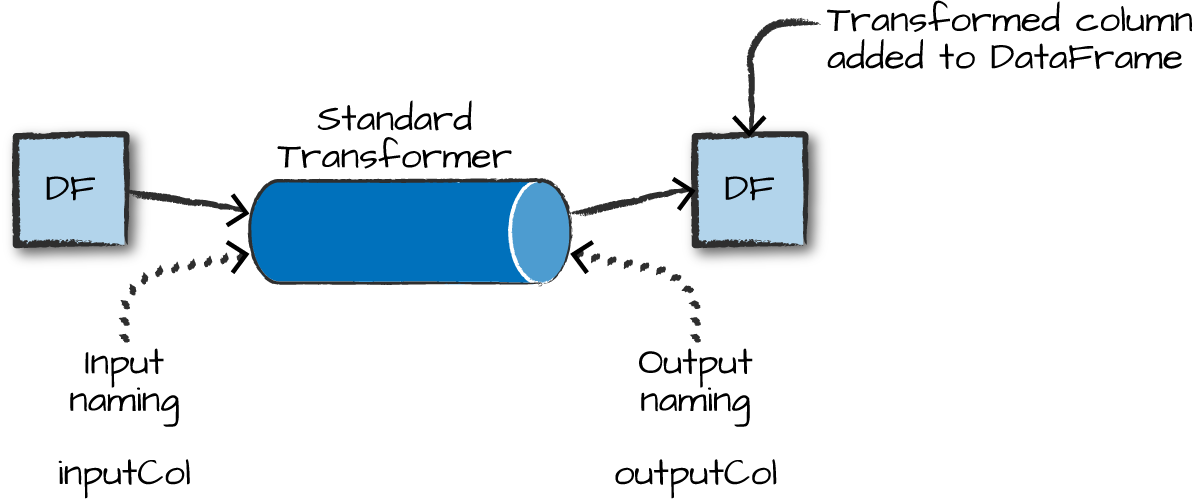
Some Examples of Transformers

Converting categorical variables to numeric (must do this)
- StringIndexer
- OneHotEncoder can act on multiple columns at a time
Data Normalization
- Normalizer
- StandardScaler
String Operations
- Tokenizer
- StopWordsRemover
- PCA
Converting continuous to discrete
- Bucketizer
- QuantileDiscretizer
Many more
- https://spark.apache.org/docs/latest/ml-guide.html

`MLlib` algorithms for machine learning models need single, numeric features column as input

Each row in this column contains a vector of data points corresponding to the set of features used for prediction.

Use the VectorAssembler transformer to create a single vector column from a list of columns.
All categorical data needs to be numeric for machine learning

# Example from Spark docs
from pyspark.ml.linalg import Vectors
from pyspark.ml.feature import VectorAssembler

dataset = spark.createDataFrame(
    [(0, 18, 1.0, Vectors.dense([0.0, 10.0, 0.5]), 1.0)],
    ["id", "hour", "mobile", "userFeatures", "clicked"])

assembler = VectorAssembler(
    inputCols=["hour", "mobile", "userFeatures"],
    outputCol="features")

output = assembler.transform(dataset)
print("Assembled columns 'hour', 'mobile', 'userFeatures' to vector column 'features'")
output.select("features", "clicked").show(truncate=False)

Estimators

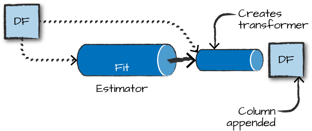
Estimators learn (or “fit”) parameters from your DataFrame via the .fit() method, and return a model which is a Transformer

Pipelines

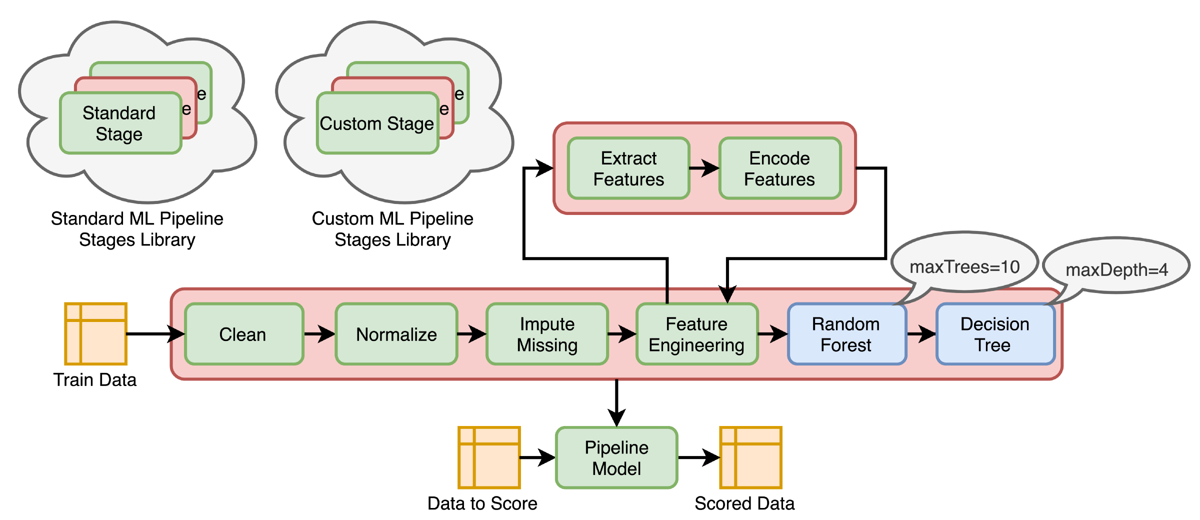
Pipelines combine multiple steps into a single workflow that can be easily run. * Data cleaning and feature processing via transformers, using stages * Model definition * Run the pipeline to do all transformations and fit the model

The Pipeline constructor takes an array of pipeline stages

Why Pipelines?

Cleaner Code: Accounting for data at each step of preprocessing can get messy. With a Pipeline, you won’t need to manually keep track of your training and validation data at each step.
Fewer Bugs: There are fewer opportunities to misapply a step or forget a preprocessing step.
Easier to Productionize: It can be surprisingly hard to transition a model from a prototype to something deployable at scale, but Pipelines can help.
More Options for Model Validation: We can easily apply cross-validation and other techniques to our Pipelines.

Example

Using the HMP Dataset. The structure of the dataset looks like this:

# read data from text file and split each line into words
df.printSchema()

root  
|-- x: integer (nullable = true)  
|-- y: integer (nullable = true)  
|-- z: integer (nullable = true)  
|-- class: string (nullable = false)  
|-- source: string (nullable = false)

Let’s transform strings into numbers

The StringIndexer is an estimator having both fit and transform methods.
To create a StringIndexer object (indexer), pass the class column as inputCol, and classIndex as outputCol.
Then we fit the DataFrame to the indexer (running the estimator), and transform the DataFrame (running the transformer). This creates a brand new DataFrame (indexed), which we can see below, containing the classIndex additional column.

from pyspark.ml.feature import StringIndexer

indexer = StringIndexer(inputCol = 'class', outputCol = 'classIndex')
indexed = indexer.fit(df).transform(df)  # This is a new data frame

# Let's see it
indexed.show(5)

+---+---+---+-----------+--------------------+----------+
|  x|  y|  z|      class|              source|classIndex|
+---+---+---+-----------+--------------------+----------+
| 29| 39| 51|Drink_glass|Accelerometer-201...|       2.0|
| 29| 39| 51|Drink_glass|Accelerometer-201...|       2.0|
| 28| 38| 52|Drink_glass|Accelerometer-201...|       2.0|
| 29| 37| 51|Drink_glass|Accelerometer-201...|       2.0|
| 30| 38| 52|Drink_glass|Accelerometer-201...|       2.0|
+---+---+---+-----------+--------------------+----------+
only showing top 5 rows

One-Hot Encode categorical variables

Unlike the StringIndexer, OneHotEncoder is a pure transformer, having only the transform method. It uses the same syntax of inputCol and outputCol.
OneHotEncoder creates a brand new DataFrame (encoded), with a category_vec column added to the previous DataFrame(indexed).
OneHotEncoder doesn’t return several columns containing only zeros and ones; it returns a sparse-vector as seen in the categoryVec column. Thus, for the ‘Drink_glass’ class above, SparkML returns a sparse-vector that says there are 13 elements, and at position 2, the class value exists(1.0).

from pyspark.ml.feature import OneHotEncoder

# The OneHotEncoder is a pure transformer object. it does not use the fit()
encoder = OneHotEncoder(inputCol = 'classIndex', outputCol = 'categoryVec')
encoded = encoder.transform(indexed)  # This is a new data frame
encoded.show(5, False)

+---+---+---+-----------+----------------------------------------------------+----------+--------------+
|x  |y  |z  |class      |source                                              |classIndex|categoryVec   |
+---+---+---+-----------+----------------------------------------------------+----------+--------------+
|29 |39 |51 |Drink_glass|Accelerometer-2011-06-01-14-13-57-drink_glass-f1.txt|2.0       |(13,[2],[1.0])|
|29 |39 |51 |Drink_glass|Accelerometer-2011-06-01-14-13-57-drink_glass-f1.txt|2.0       |(13,[2],[1.0])|
|28 |38 |52 |Drink_glass|Accelerometer-2011-06-01-14-13-57-drink_glass-f1.txt|2.0       |(13,[2],[1.0])|
|29 |37 |51 |Drink_glass|Accelerometer-2011-06-01-14-13-57-drink_glass-f1.txt|2.0       |(13,[2],[1.0])|
|30 |38 |52 |Drink_glass|Accelerometer-2011-06-01-14-13-57-drink_glass-f1.txt|2.0       |(13,[2],[1.0])|
+---+---+---+-----------+----------------------------------------------------+----------+--------------+
only showing top 5 rows

Assembling the feature vector

The VectorAssembler object gets initialized with the same syntax as StringIndexer and OneHotEncoder.
The list ['x', 'y', 'z'] is passed to inputCols, and we specify outputCol = ‘features’.
This is also a pure transformer.

from pyspark.ml.linalg import Vectors
from pyspark.ml.feature import VectorAssembler
# VectorAssembler creates vectors from ordinary data types for us

vectorAssembler = VectorAssembler(inputCols = ['x','y','z'], outputCol = 'features')
# Now we use the vectorAssembler object to transform our last updated dataframe

features_vectorized = vectorAssembler.transform(encoded)  # note this is a new df

features_vectorized.show(5, False)

+---+---+---+-----------+----------------------------------------------------+----------+--------------+----------------+
|x  |y  |z  |class      |source                                              |classIndex|categoryVec   |features        |
+---+---+---+-----------+----------------------------------------------------+----------+--------------+----------------+
|29 |39 |51 |Drink_glass|Accelerometer-2011-06-01-14-13-57-drink_glass-f1.txt|2.0       |(13,[2],[1.0])|[29.0,39.0,51.0]|
|29 |39 |51 |Drink_glass|Accelerometer-2011-06-01-14-13-57-drink_glass-f1.txt|2.0       |(13,[2],[1.0])|[29.0,39.0,51.0]|
|28 |38 |52 |Drink_glass|Accelerometer-2011-06-01-14-13-57-drink_glass-f1.txt|2.0       |(13,[2],[1.0])|[28.0,38.0,52.0]|
|29 |37 |51 |Drink_glass|Accelerometer-2011-06-01-14-13-57-drink_glass-f1.txt|2.0       |(13,[2],[1.0])|[29.0,37.0,51.0]|
|30 |38 |52 |Drink_glass|Accelerometer-2011-06-01-14-13-57-drink_glass-f1.txt|2.0       |(13,[2],[1.0])|[30.0,38.0,52.0]|
+---+---+---+-----------+----------------------------------------------------+----------+--------------+----------------+
only showing top 5 rows

Normalizing the dataset

Normalizer, like all transformers, has a consistent syntax. Looking at the Normalizer object, it contains the parameter p=1.0 (the default norm value for Pyspark Normalizer is p=2.0.)
p=1.0 uses Manhattan Distance
p=2.0 uses Euclidean Distance

from pyspark.ml.feature import Normalizer
normalizer = Normalizer(inputCol = 'features', outputCol = 'features_norm', p=1.0)  # Manhattan Distance
normalized_data = normalizer.transform(features_vectorized) # New data frame too.

normalized_data.show(5)
>>
+---+---+---+-----------+--------------------+----------+--------------+----------------+--------------------+
|  x|  y|  z|      class|              source|classIndex|   categoryVec|        features|       features_norm|
+---+---+---+-----------+--------------------+----------+--------------+----------------+--------------------+
| 29| 39| 51|Drink_glass|Accelerometer-201...|       2.0|(13,[2],[1.0])|[29.0,39.0,51.0]|[0.24369747899159...|
| 29| 39| 51|Drink_glass|Accelerometer-201...|       2.0|(13,[2],[1.0])|[29.0,39.0,51.0]|[0.24369747899159...|
| 28| 38| 52|Drink_glass|Accelerometer-201...|       2.0|(13,[2],[1.0])|[28.0,38.0,52.0]|[0.23728813559322...|
| 29| 37| 51|Drink_glass|Accelerometer-201...|       2.0|(13,[2],[1.0])|[29.0,37.0,51.0]|[0.24786324786324...|
| 30| 38| 52|Drink_glass|Accelerometer-201...|       2.0|(13,[2],[1.0])|[30.0,38.0,52.0]|[0.25,0.316666666...|
+---+---+---+-----------+--------------------+----------+--------------+----------------+--------------------+
only showing top 5 rows

Running the transformation `Pipeline`

The Pipeline constructor below takes an array of Pipeline stages we pass to it. Here we pass the 4 stages defined earlier, in the right sequence, one after another.

from pyspark.ml import Pipeline
pipeline = Pipeline(stages = [indexer,encoder,vectorAssembler,normalizer])

Now the Pipeline object fits to our original DataFrame df

data_model = pipeline.fit(df)

Finally, we transform our DataFrame df using the Pipeline Object.

pipelined_data = data_model.transform(df)

pipelined_data.show(5)

+---+---+---+-----------+--------------------+----------+--------------+----------------+--------------------+
|  x|  y|  z|      class|              source|classIndex|   categoryVec|        features|       features_norm|
+---+---+---+-----------+--------------------+----------+--------------+----------------+--------------------+
| 29| 39| 51|Drink_glass|Accelerometer-201...|       2.0|(13,[2],[1.0])|[29.0,39.0,51.0]|[0.24369747899159...|
| 29| 39| 51|Drink_glass|Accelerometer-201...|       2.0|(13,[2],[1.0])|[29.0,39.0,51.0]|[0.24369747899159...|
| 28| 38| 52|Drink_glass|Accelerometer-201...|       2.0|(13,[2],[1.0])|[28.0,38.0,52.0]|[0.23728813559322...|
| 29| 37| 51|Drink_glass|Accelerometer-201...|       2.0|(13,[2],[1.0])|[29.0,37.0,51.0]|[0.24786324786324...|
| 30| 38| 52|Drink_glass|Accelerometer-201...|       2.0|(13,[2],[1.0])|[30.0,38.0,52.0]|[0.25,0.316666666...|
+---+---+---+-----------+--------------------+----------+--------------+----------------+--------------------+
only showing top 5 rows

One last step before training

# first let's list out the columns we want to drop
cols_to_drop = ['x','y','z','class','source','classIndex','features']

# Next let's use a list comprehension with conditionals to select cols we need
selected_cols = [col for col in pipelined_data.columns if col not in cols_to_drop]

# Let's define a new train_df with only the categoryVec and features_norm cols
df_train = pipelined_data.select(selected_cols)

# Let's see our training dataframe.
df_train.show(5)

+--------------+--------------------+
|   categoryVec|       features_norm|
+--------------+--------------------+
|(13,[2],[1.0])|[0.24369747899159...|
|(13,[2],[1.0])|[0.24369747899159...|
|(13,[2],[1.0])|[0.23728813559322...|
|(13,[2],[1.0])|[0.24786324786324...|
|(13,[2],[1.0])|[0.25,0.316666666...|
only showing top 5 rows

You now have a DataFrame optimized for SparkML!

Machine Learning Models in Spark

There are many Spark machine learning models

Regression

Linear regression - what is the optimization method?
Survival regression
Generalized linear model (GLM)
Random forest regression

Classification

Logistic regression
Gradient-boosted tree model (GBM)
Naive Bayes
Multilayer perception (neural network!)

Other

Clustering (K-means, LDA, GMM)
Association rule mining

Building your Model

Feature selection using easy R-like formulas

# Example from Spark docs
from pyspark.ml.feature import RFormula

dataset = spark.createDataFrame(
    [(7, "US", 18, 1.0),
     (8, "CA", 12, 0.0),
     (9, "NZ", 15, 0.0)],
    ["id", "country", "hour", "clicked"])

formula = RFormula(
    formula="clicked ~ country + hour",
    featuresCol="features",
    labelCol="label")

output = formula.fit(dataset).transform(dataset)
output.select("features", "label").show()

What if you have too many columns for your model?

Evaluating 1,000s or 10,000s of variables?

Chi-Squared Selector

Pick categorical variables that are most dependent on the response variable

Can even check the p-values of specific variables!

# Example from Spark docs
from pyspark.ml.feature import ChiSqSelector
from pyspark.ml.linalg import Vectors

df = spark.createDataFrame([
    (7, Vectors.dense([0.0, 0.0, 18.0, 1.0]), 1.0,),
    (8, Vectors.dense([0.0, 1.0, 12.0, 0.0]), 0.0,),
    (9, Vectors.dense([1.0, 0.0, 15.0, 0.1]), 0.0,)], ["id", "features", "clicked"])

selector = ChiSqSelector(numTopFeatures=1, featuresCol="features",
                         outputCol="selectedFeatures", labelCol="clicked")

result = selector.fit(df).transform(df)

print("ChiSqSelector output with top %d features selected" % selector.getNumTopFeatures())
result.show()

Tuning your model

Part 1

# Example from Spark docs
from pyspark.ml.evaluation import RegressionEvaluator
from pyspark.ml.regression import LinearRegression
from pyspark.ml.tuning import ParamGridBuilder, TrainValidationSplit

# Prepare training and test data.
data = spark.read.format("libsvm")\
    .load("data/mllib/sample_linear_regression_data.txt")
train, test = data.randomSplit([0.9, 0.1], seed=12345)

lr = LinearRegression(maxIter=10)

# We use a ParamGridBuilder to construct a grid of parameters to search over.
# TrainValidationSplit will try all combinations of values and determine best model using
# the evaluator.
paramGrid = ParamGridBuilder()\
    .addGrid(lr.regParam, [0.1, 0.01]) \
    .addGrid(lr.fitIntercept, [False, True])\
    .addGrid(lr.elasticNetParam, [0.0, 0.5, 1.0])\
    .build()

Tuning your model

Part 2

# In this case the estimator is simply the linear regression.
# A TrainValidationSplit requires an Estimator, a set of Estimator ParamMaps, and an Evaluator.
tvs = TrainValidationSplit(estimator=lr,
                           estimatorParamMaps=paramGrid,
                           evaluator=RegressionEvaluator(),
                           # 80% of the data will be used for training, 20% for validation.
                           trainRatio=0.8)

# Run TrainValidationSplit, and choose the best set of parameters.
model = tvs.fit(train)

# Make predictions on test data. model is the model with combination of parameters
# that performed best.
model.transform(test)\
    .select("features", "label", "prediction")\
    .show()

Project Review

Review project overview https://gu-dsan.github.io/6000-fall-2023/project/project.html

Assignment link - https://georgetown.instructure.com/courses/172712/assignments/958317

Lecture 9

Logistics and Review

Deadlines

Look back and ahead

Review of Prior Topics

AWS Academy

Caching and Persistence

collect CAUTION

Assumption: knowledge of ML techniques and process

Overview of ML

The advanced analytics/ML process

ML with Spark

What is MLlib

Capabilities

API is divided into two packages

Inspired by scikit-learn

Transformers, estimators, and pipelines

Transformers

Some Examples of Transformers

MLlib algorithms for machine learning models need single, numeric features column as input

Estimators

Pipelines

Pipelines

Why Pipelines?

Example

Let’s transform strings into numbers

One-Hot Encode categorical variables

Assembling the feature vector

Normalizing the dataset

Running the transformation Pipeline

One last step before training

You now have a DataFrame optimized for SparkML!

Machine Learning Models in Spark

Regression

Classification

Other

Building your Model

What if you have too many columns for your model?

Chi-Squared Selector

Tuning your model

Part 1

Tuning your model

Part 2

Project Review

Lab time!

`collect` CAUTION

What is `MLlib`

Inspired by `scikit-learn`

`MLlib` algorithms for machine learning models need single, numeric features column as input

Running the transformation `Pipeline`