| Term | Definition |
|---|---|
| Local | Your current workstation (laptop, desktop, etc.), wherever you start the terminal/console application. |
| Remote | Any machine you connect to via ssh or other means. |
| EC2 | Single virtual machine in the cloud where you can run computation (ephemeral) |
| SageMaker | Integrated Developer Environment where you can conduct data science on single machines |
| Ephemeral | Lasting for a short time - any machine that will get turned off or place you will lose data |
| Persistent | Lasting for a long time - any environment where your work is NOT lost when the timer goes off |
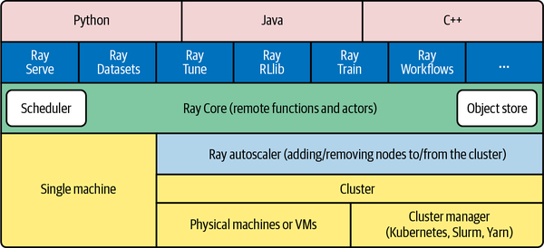
Lecture 3
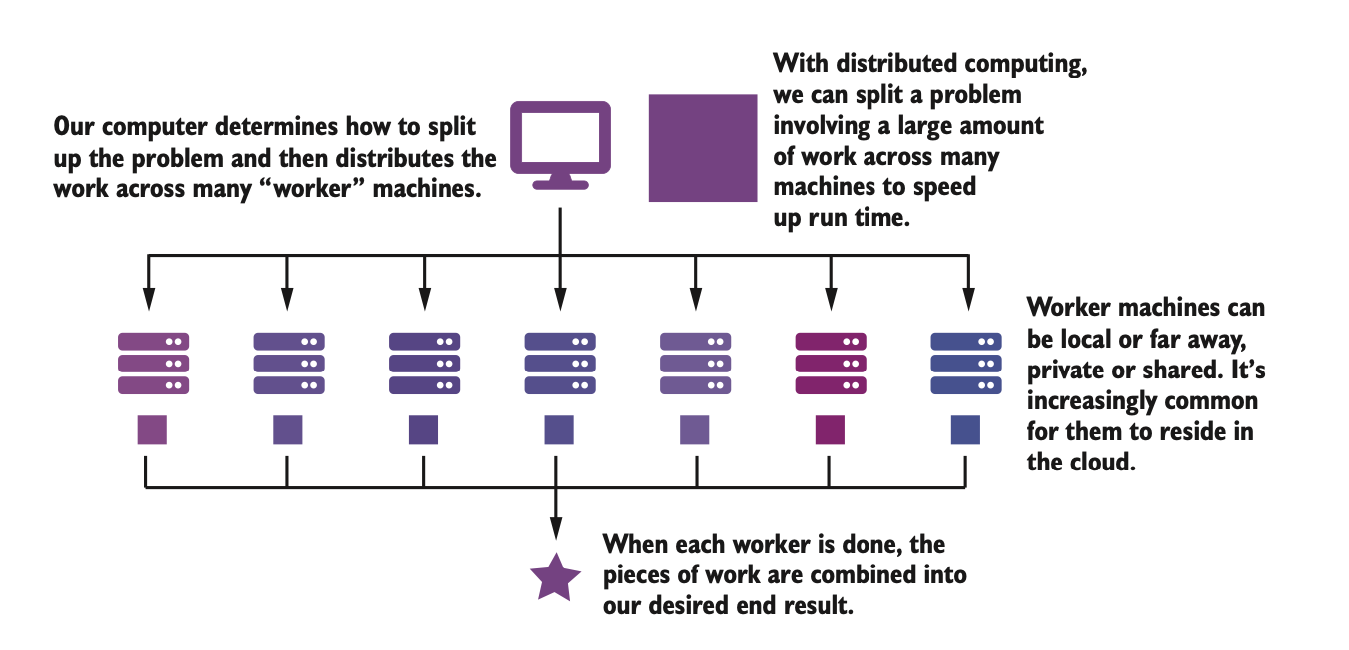
Parallelization, map & reduce functions
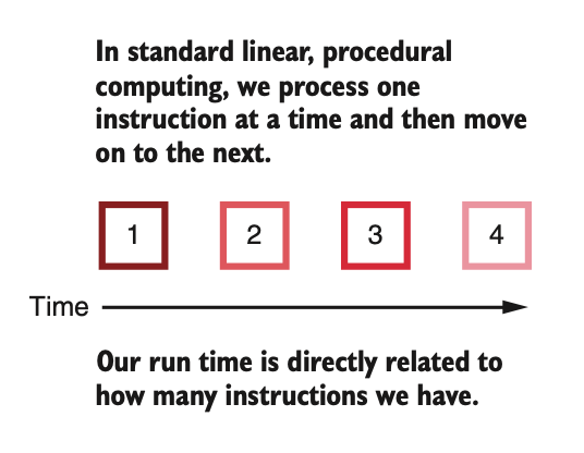
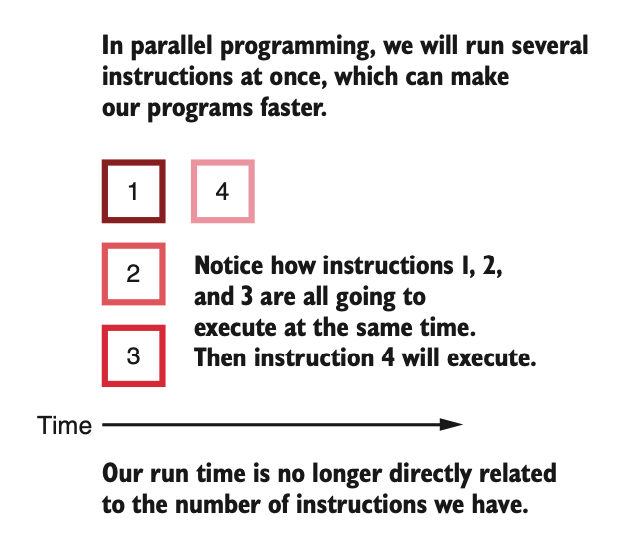
Linear vs. Parallel
Amdahl’s Law

\[ \lim_{s\rightarrow\infty} S_{latency} = \frac{1}{1-p} \]
where \(s\) is the speedup of that part of the task (which is \(p\) proportion of the overall task) benefitting from improved resources.
If 50% of the task is embarassingly parallel, you can get a maximum speedup of 2-fold, while if 90% is embarassingly parallel, you can get a maximum speedup of \(1/(1-0.9) = 10\) fold.
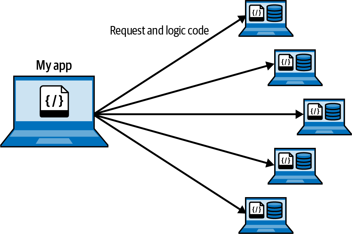
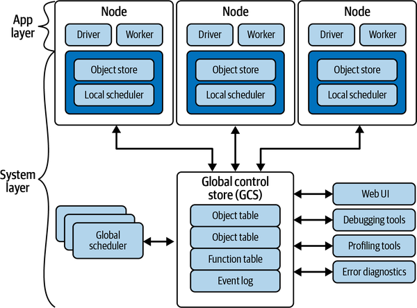
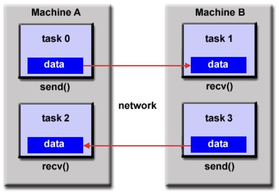
Distributed memory / Message Passing Model
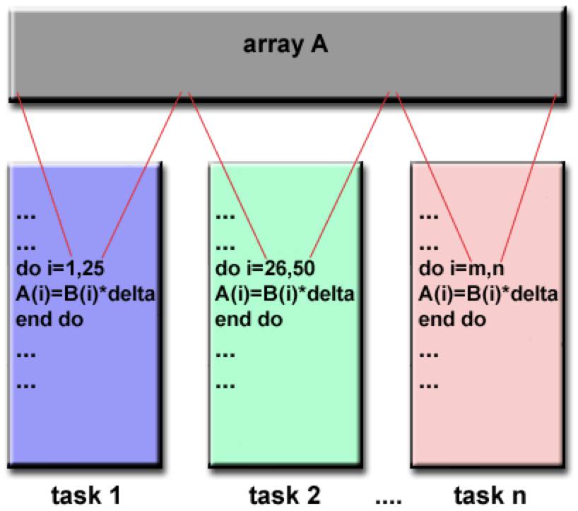
Data parallel model
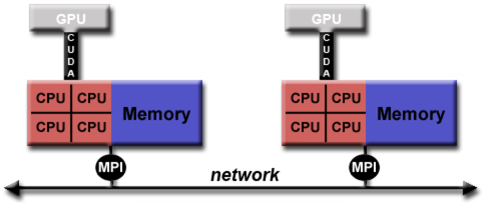
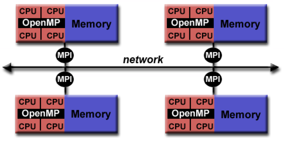
Hybrid model
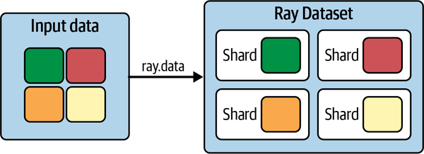
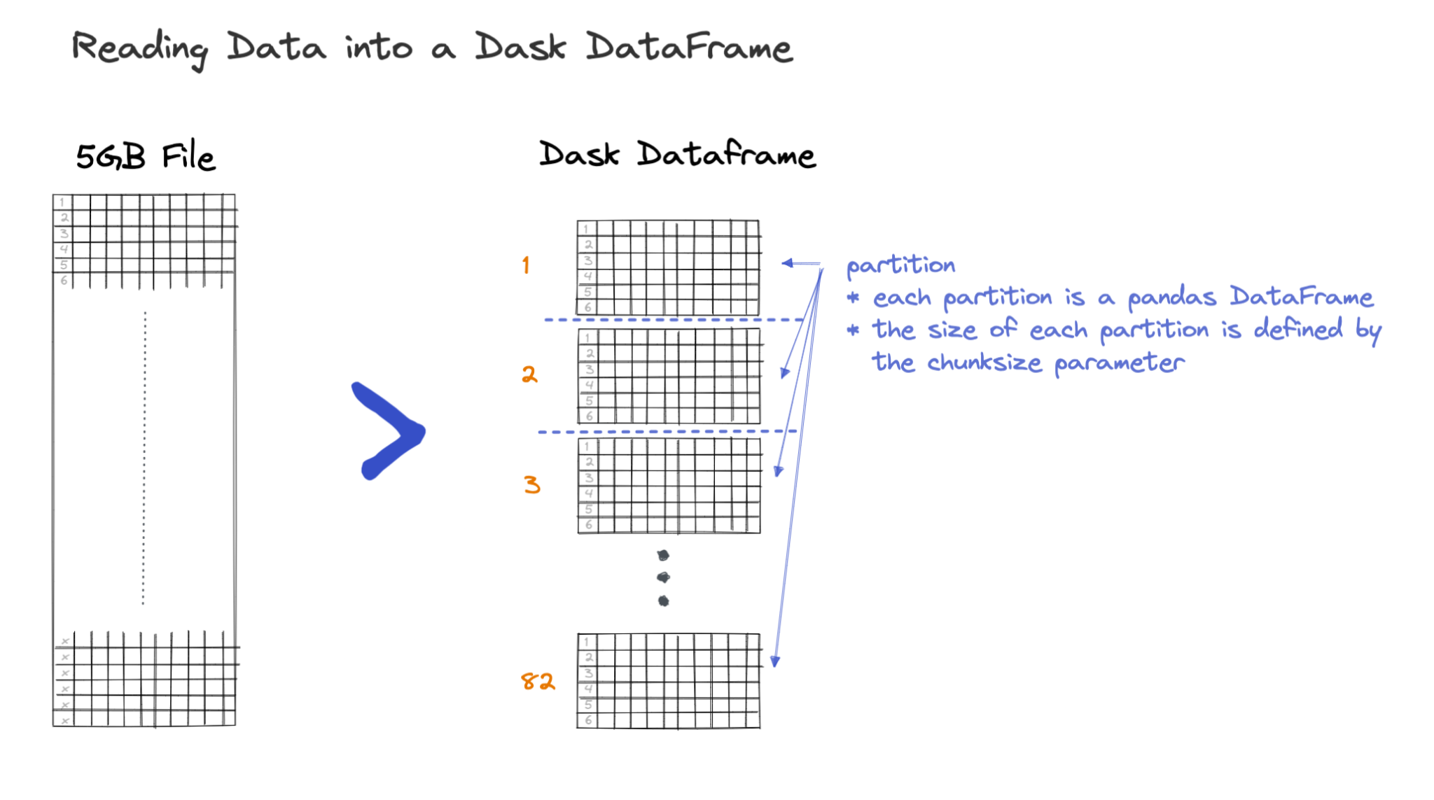
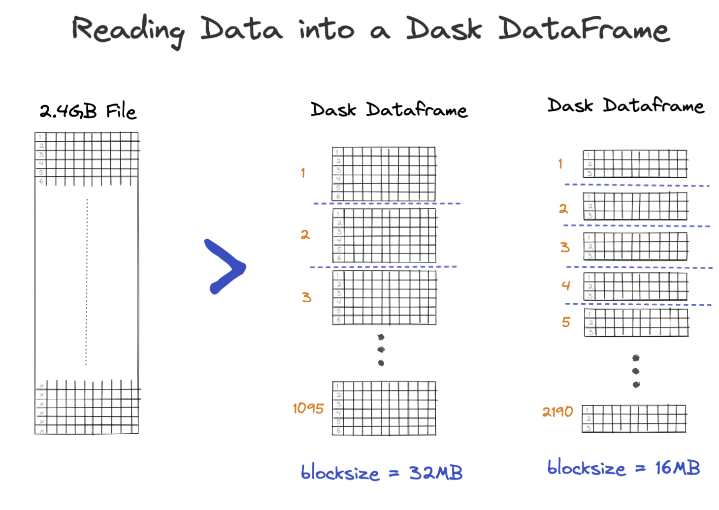
Partitioning data
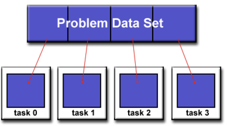
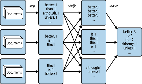
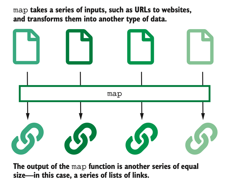
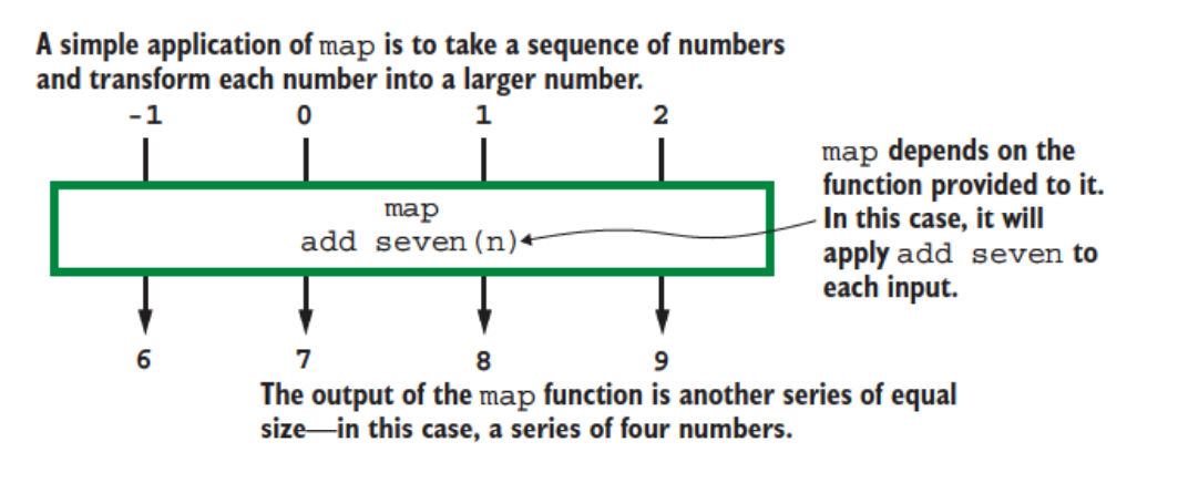
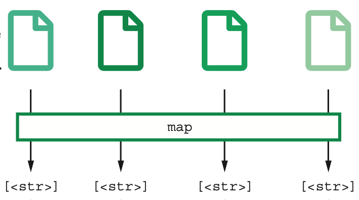
Map
The map operation is a 1-1 operation that takes each split and processes it
The map operation keeps the same number of objects in its output that were present in its input
Map
The operations included in a particular map can be quite complex, involving multiple steps. In fact, you can implement a pipeline of procedures within the map step to process each data object.
The main point is that the same operations will be run on each data object in the map implementation
Map
Some examples of a map operations are
- Extracting a standard table from online reports from multiple years
- Extracting particular records from multiple JSON objects
- Transforming data (as opposed to summarizing it)
- Run a normalization script on each transcript in a GWAS dataset
- Standardizing demographic data for each of the last 20 years against the 2000 US population
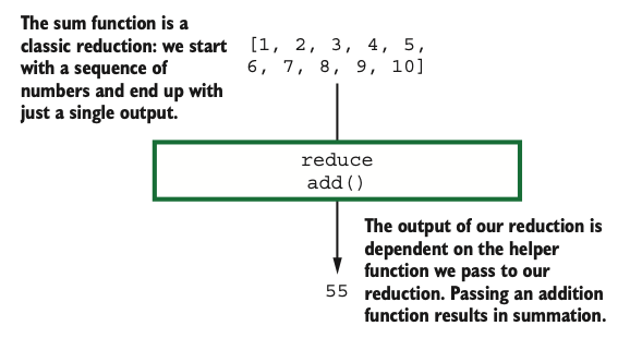
Reduce
The reduce operation takes multiple objects and reduces them to a (perhaps) smaller number of objects using transformations that aren’t amenable to the map paradigm.
These transformations are often serial/linear in nature
The reduce transformation is usually the last, not-so-elegant transformation needed after most of the other transformations have been efficiently handled in a parallel fashion by map
Reduce
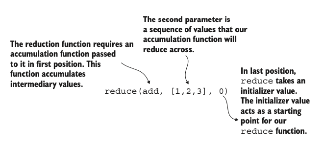
The reduce operation requires
- An accumulator function, that will update serially as new data is fed into it
- A sequence of objects to run through the accumulator function
- A starting value from which the accumulator function starts
Programmatically, this can be written as
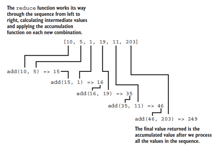
Reduce
The reduce operation works serially from “left” to “right”, passing each object successively through the accumulator function.
For example, if we were to add successive numbers with a function called add…
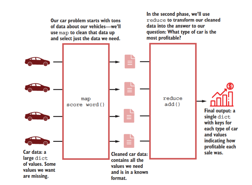
map-reduce
Combining the map and reduce operations creates a powerful pipeline that can handle a diverse range of problems in the Big Data context
Parallelization and map-reduce are bed-mates
One of the issues here is, how to split the data in a “good” manner so that the map-reduce framework works well
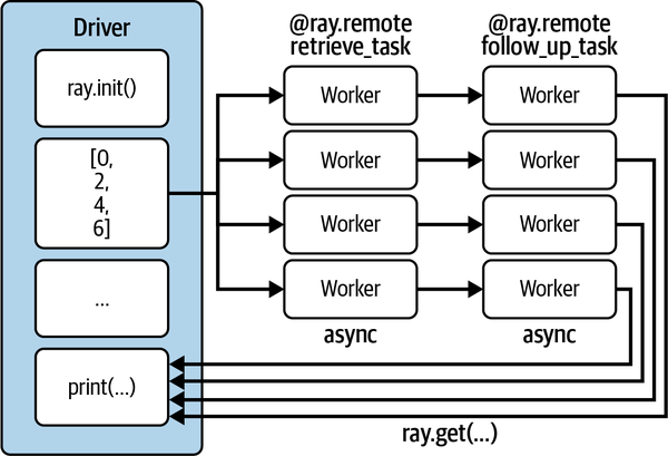
The need for Async I/O
When talking to external systems (databases, APIs) the bottleneck is not local CPU/memory but rather the time it takes to receive a response from the external system.
The Async I/O model addresses this by allowing to send multiple request in parallel without having to wait for a response.
References: asyncio — Asynchronous I/O, Async IO in Python: A Complete Walkthrough

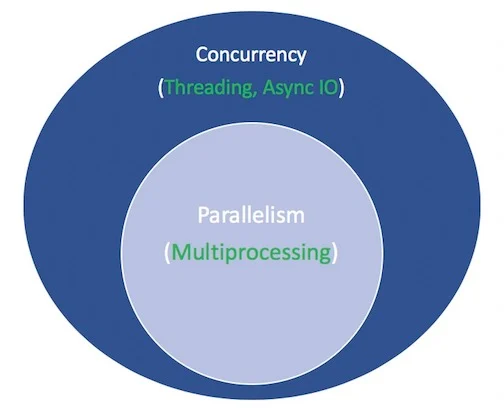
Concurrency and parallelism in Python3
Parallelism: multiple tasks are running in parallel, each on a different processors. This is done through the
multiprocessingmodule.Concurrency: multiple tasks are taking turns to run on the same processor. Another task can be scheduled while the current one is blocked on I/O.
Threading: multiple threads take turns executing tasks. One process can contain multiple threads. Similar to concurrency but within the context of a single process.