Lecture 7
Maps and geospatial data, working with coordinate systems and projections
Reviewing data types
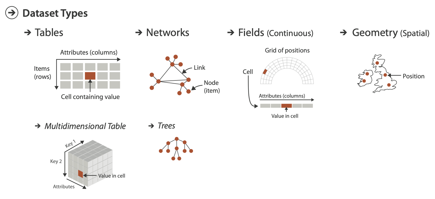
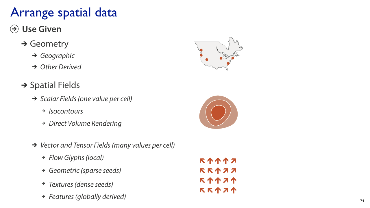
Let’s focus on Spatial data
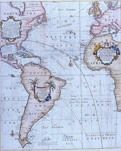
Spatial data has been around for a long time…
Edmund Halley’s New and Correct Chart Shewing the Variations of the Compass (1701) was the first map to show lines of equal magnetic variation.
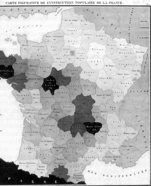
The first known instance of a choropleth
In 1826, Charles Dupin published a thematic map of France showing illiteracy levels using shadings from white to black.
A really interesting map
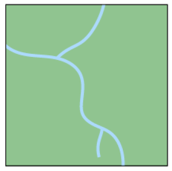
Vector Data
The geographic vector model is based on points located within a coordinate reference system (CRS). Points can represent self-standing features (e.g., the location of a bus stop) or they can be linked together to form more complex geometries such as lines and polygons. Most point geometries contain only two dimensions.
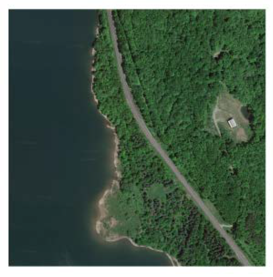
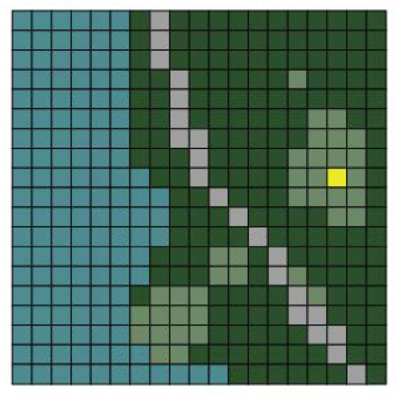
Raster Data
The geographic raster data model usually consists of a raster header and a matrix (with rows and columns) representing equally spaced cells (often called pixels).
Multi-layer Raster
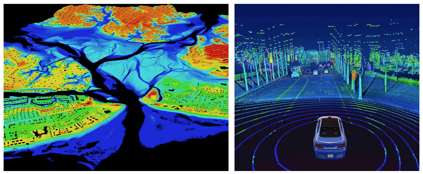
In addition to raster and vector data, there is also LiDAR data (also known as point clouds) and 3D data. LiDAR data is data that is collected via satellites, drones, or other aerial devices. 3D data is data that extends the typical latitude and longitude 2-D coordinates and incorporates elevation and or depth into the data. While complex, this data is rich with information and can be used to solve a variety of problems pertaining to the Earth’s surface.
Open Souce Libraries for GIS
GEOS (Geometry Engine - Open Source)
GEOS is a powerful geometry engine that provides functions for performing geometric operations on spatial data.
- It handles geometric objects such as points, lines, and polygons.
- Supports operations like intersection, union, buffer, and distance calculations.
- Used extensively in GIS (Geographic Information Systems) applications.
GDAL (Geospatial Data Abstraction Library)
GDAL is a versatile library for reading, writing, and transforming geospatial data.
- Handles various raster and vector formats (e.g., GeoTIFF, Shapefiles, NetCDF).
- Provides tools for data manipulation, reprojection, and format conversion.
- Supports both reading and writing of geospatial datasets.
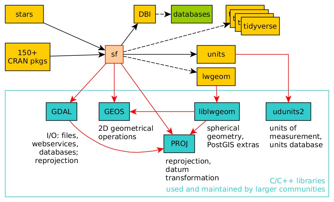
PROJ (Cartographic Projections Library)
PROJ is a library for cartographic transformations and coordinate system conversions.
- Handles coordinate reference systems (CRS) and transformations between different CRS.
- Performs accurate conversions between geographic and projected coordinates.
- Supports various map projections (e.g., Mercator, Lambert, Azimuthal).
Augmenting/Wrangling spatial data
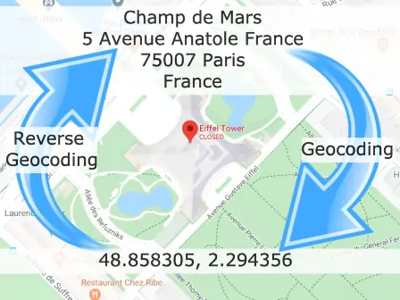
Geocoding: the process of converting an address or a name of a place into its coordinates
Reverse geocoding: the process of transforming a set of coodrinates into an address or a description of a place
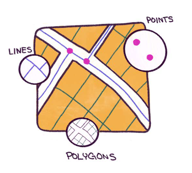
Spatial relationships
n a spatial relationships between features, each type of geometry (point, polyline, and polygon) has an interior and a boundary. How the interiors and boundaries of two geometries compare determines the spatial relationship they exhibit. The following image outlines the geometries, boundaries, and interiors of points, polylines, and polygons.

Spatial operations
Equals
A target feature is equal to a join feature if their interiors are identical and the geometry types are the same.

Planar or Geodesic Near
A target feature is within a specified distance.

Spatial operations


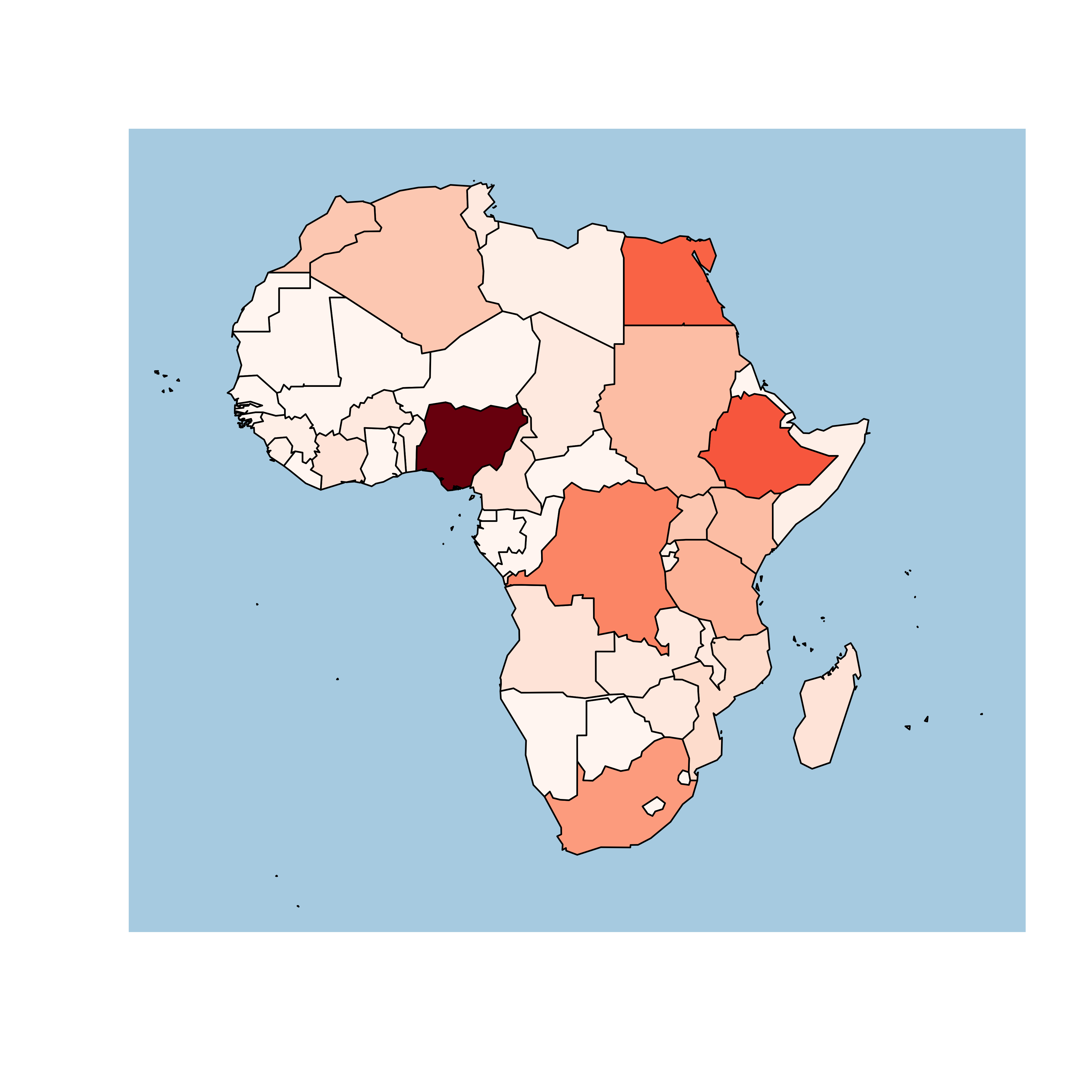
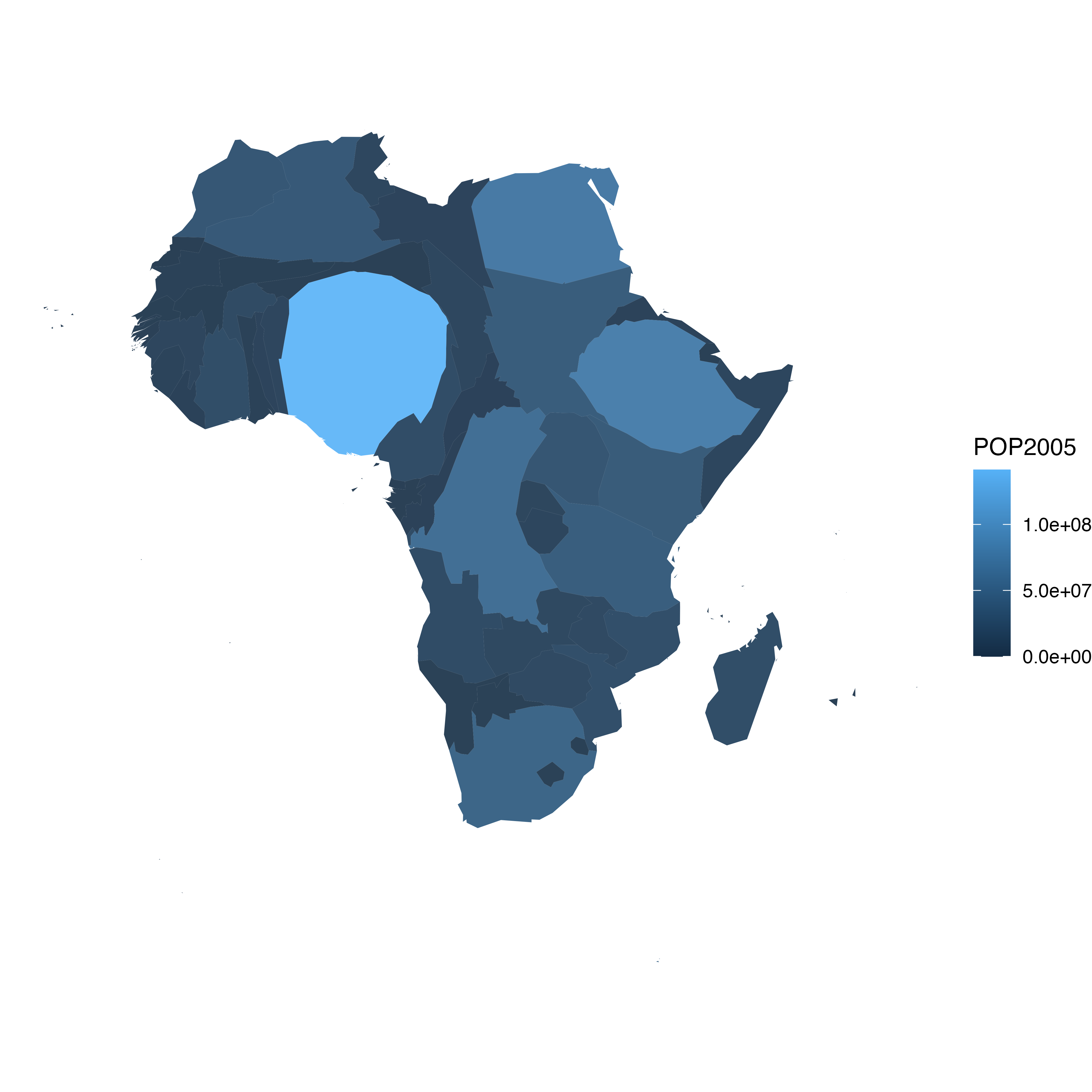
Choropleth
A choropleth map displays divided geographical areas or regions that are coloured in relation to a numeric variable.
- Use a choroplth when the main task is to undersand spatial relationships with one quantitative attribute per region
- The data is usually a table in the form of
geo,value - This is essentially a heatmap by geographic region
- Very familiar
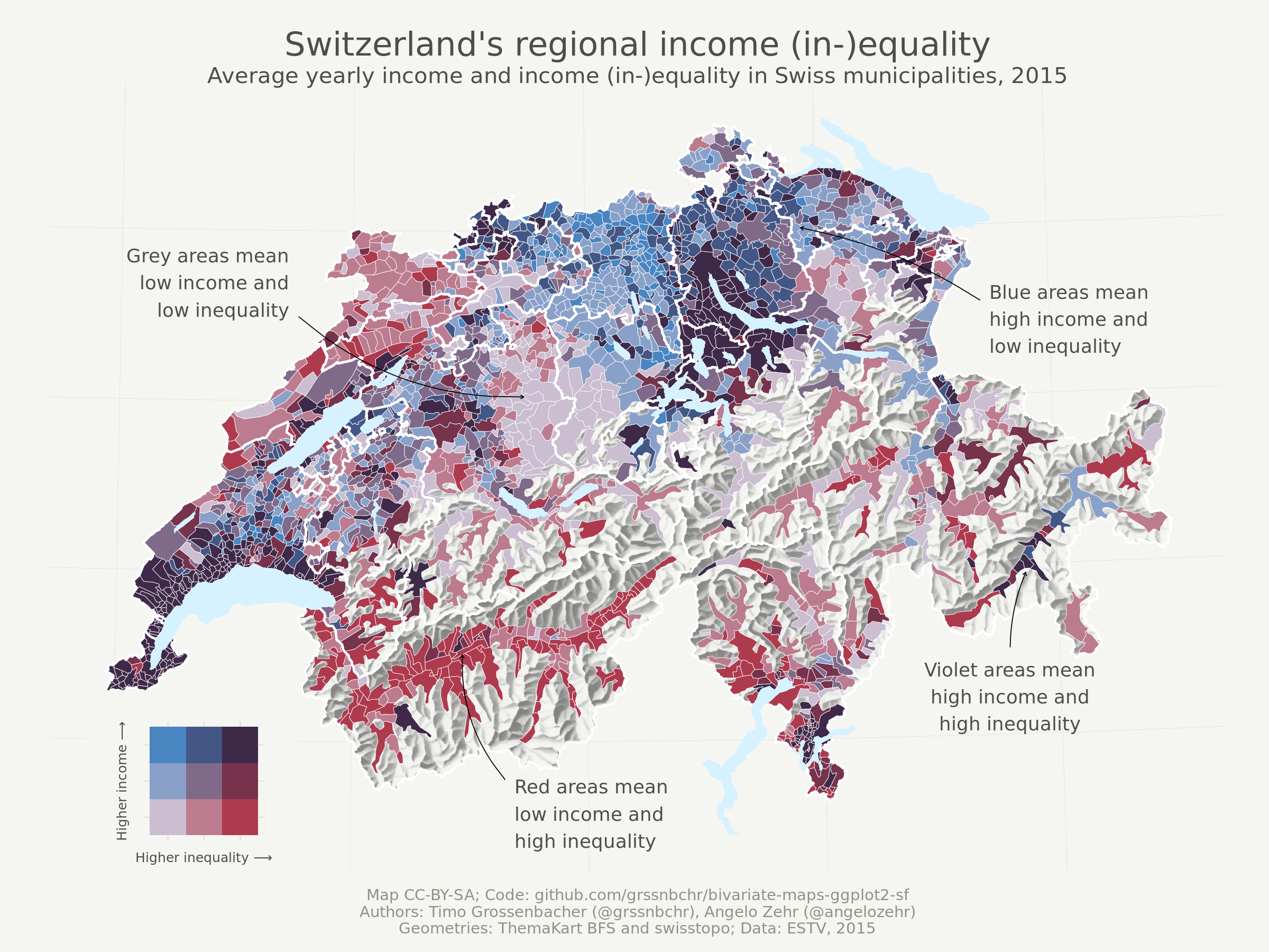
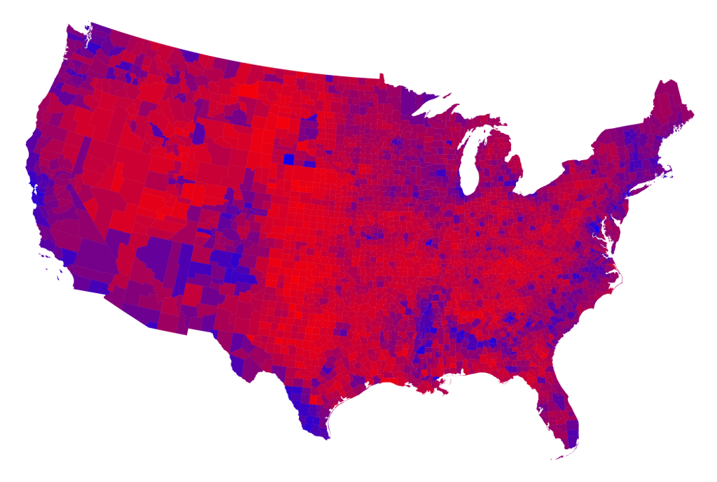
A bi-variate choropleth (using a two-level color scale)
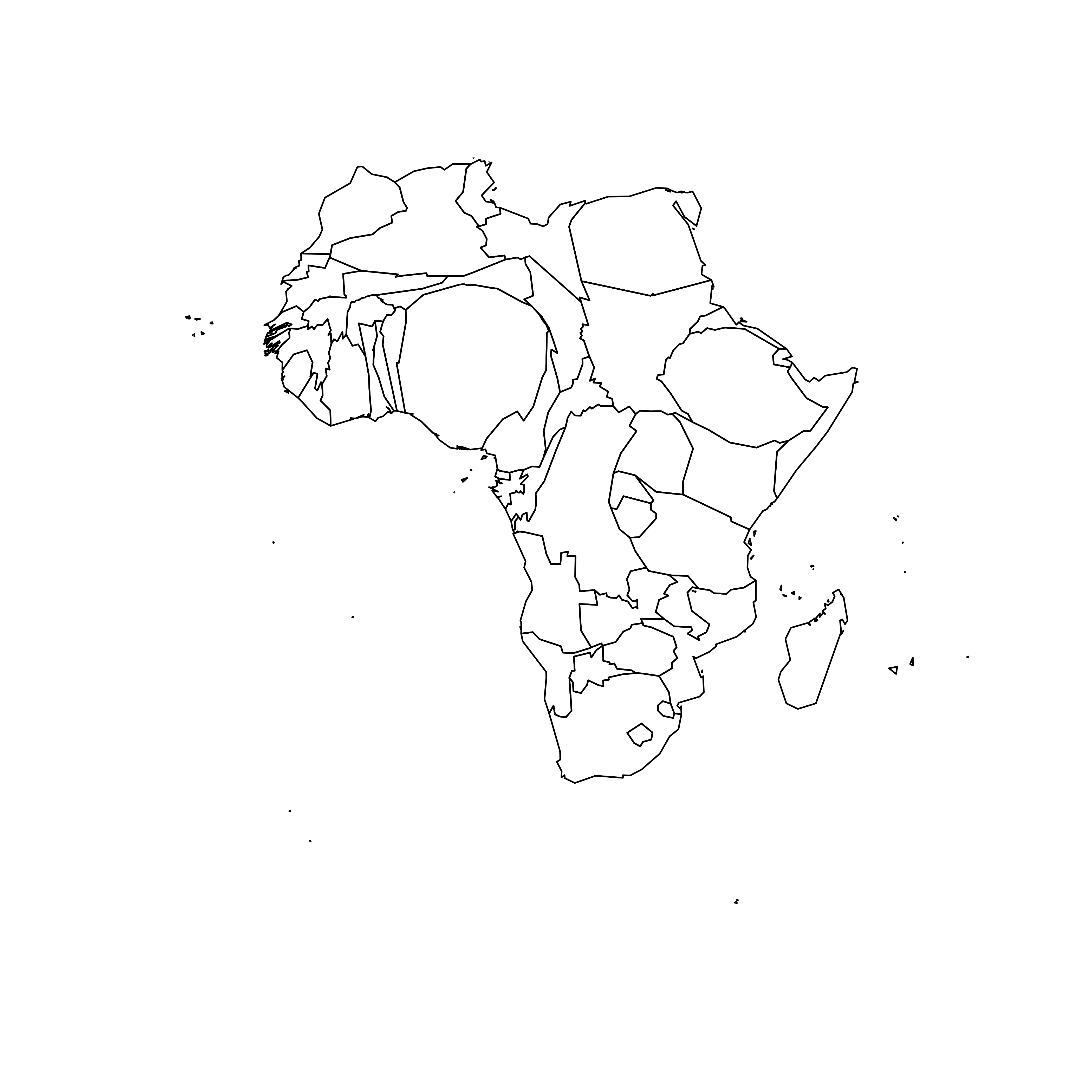
Cartogram
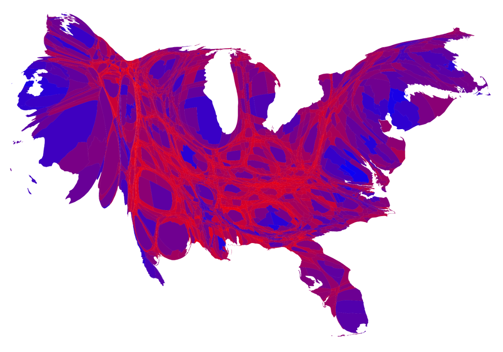
A cartogram is a map in which the geometry of regions is distorted in order to convey the information of an alternate variable. The region area will be inflated or deflated according to its numeric value.
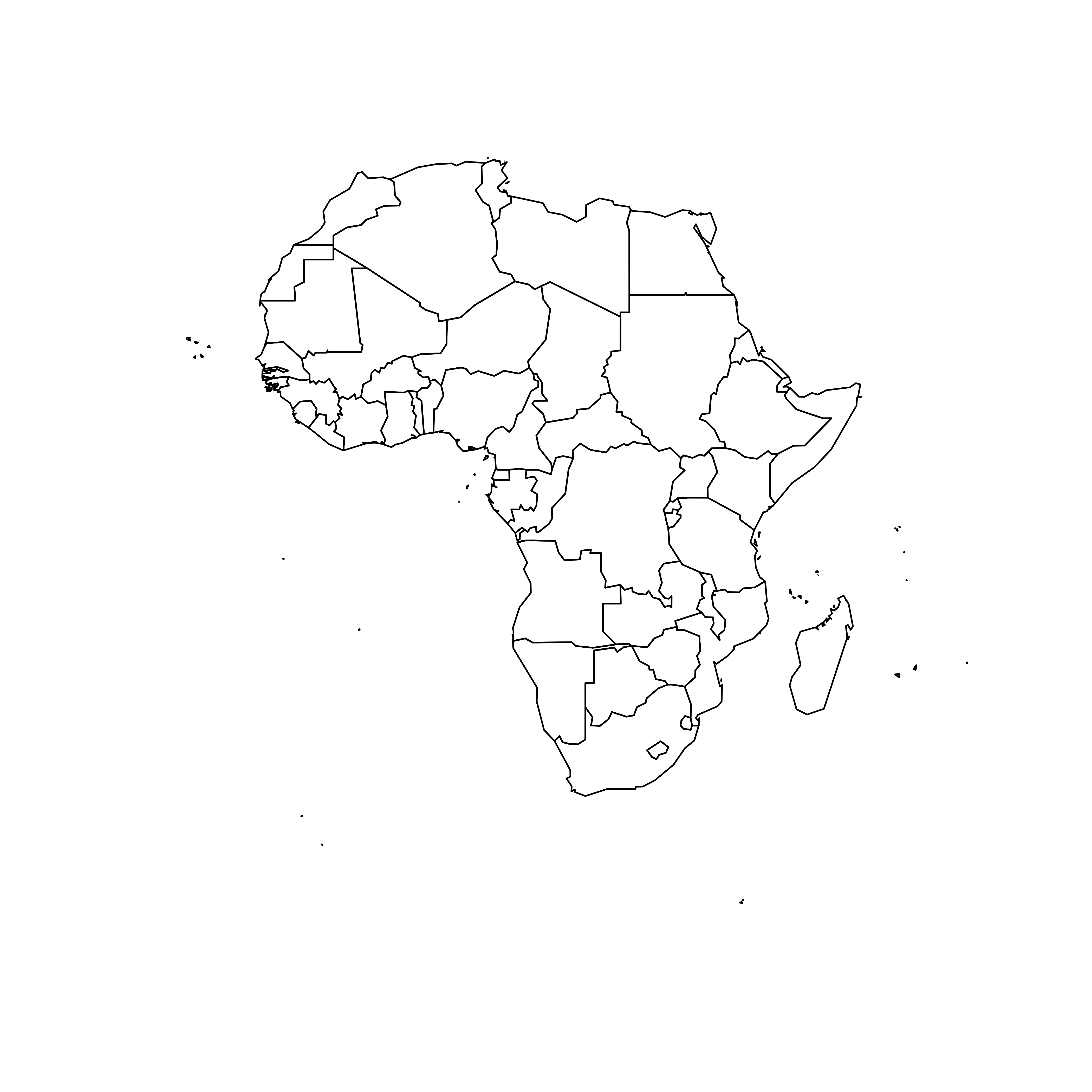
How to make a cartogram? 1. Start with the geography
Cartogram (continued)
A cartogram is a map in which the geometry of regions is distorted in order to convey the information of an alternate variable. The region area will be inflated or deflated according to its numeric value.
How to make a cartogram?
- Start with the geography
- Distort the geography based on the variable being displayed
- Add color and now you have both a choropleth and a cartogram
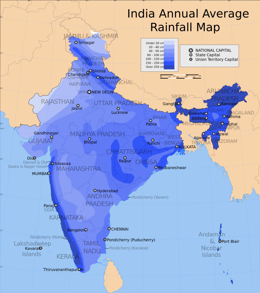
Heat maps
Heat maps are useful when you have to represent large sets of continuous data on a map using a color spectrum. A heat map is different from a chloropleth map in that the colors in a heat map do not correspond to geographical boundaries.
This map of India shows the average annual rainfall using different shades of blue. The darker the shade of blue, the higher the rainfall.
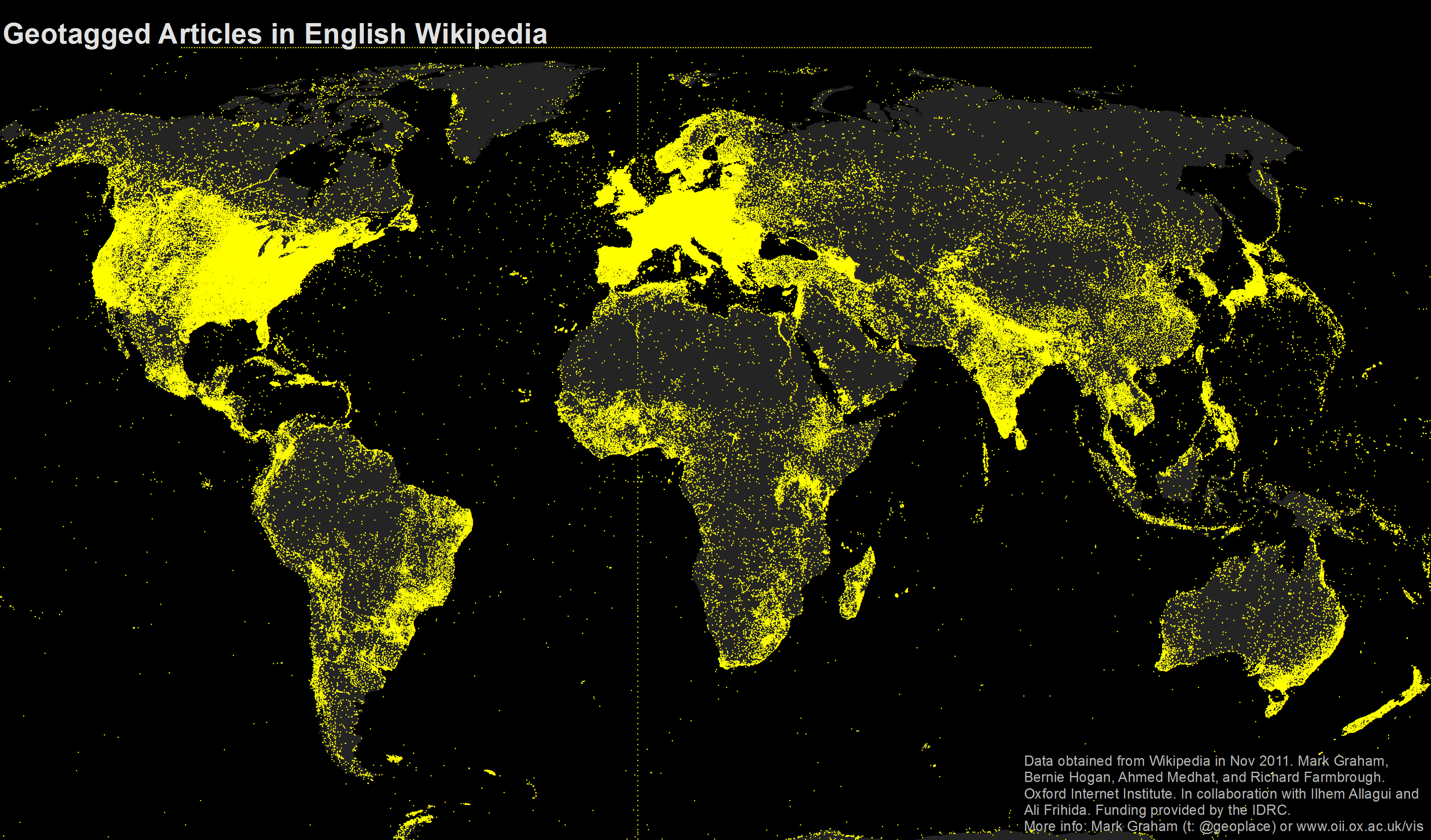
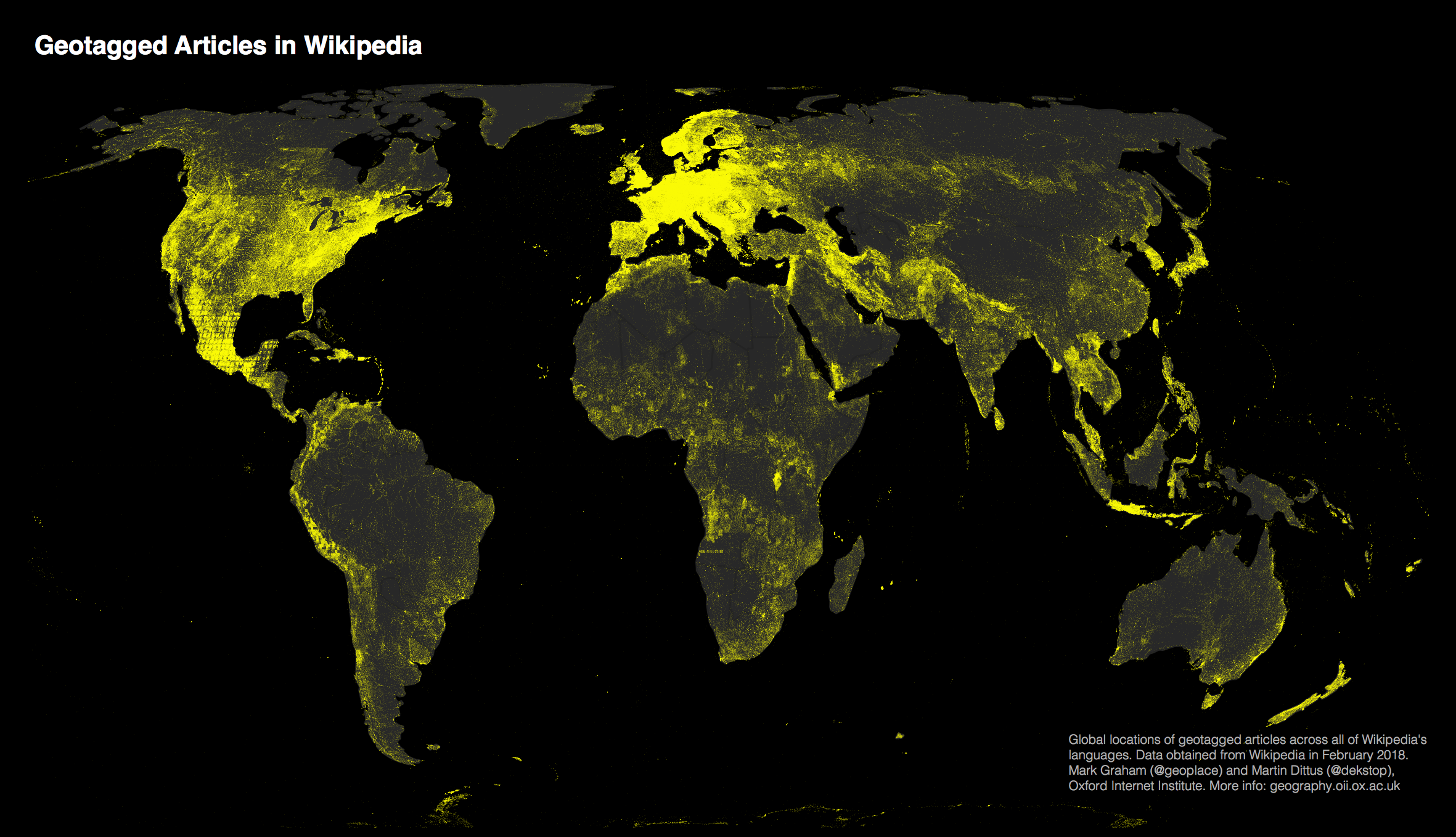
Dot map
A dot map (also called dot distribution map or dot density map) uses a dot to indicate the presence of a variable. Dot maps are essentially scatterplots on a map and are useful for showing spatial patterns.
This is a dot map of the world showing nearly 700,000 geotagged Wikipedia articles, each represented by a yellow dot, in 2011.
The same dataset, in 2018. More articles, different projections. Would you change anything?
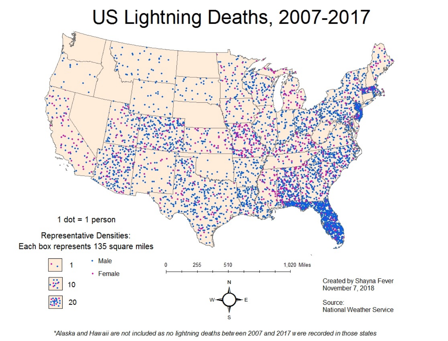
Use dot maps carefully. This is a dot density plot.
Dots are often used in graphs, charts, and maps to accurately locate individual observations and phenomena, but that’s not the case here. If you read a dot density map that way, it’ll look like there were fatalities everywhere in Florida, and that lightning strikes become much less deadly as soon as you cross the border with Georgia or Alabama.
In a dot density map, though, each dot represents one observation, but dots aren’t located where those observations were made; instead, dots are distributed to maximize coverage and, if the placement algorithm is well designed and manually tweaked, it’ll avoid absurd placement —such as dots over lakes, rivers, or unpopulated regions.
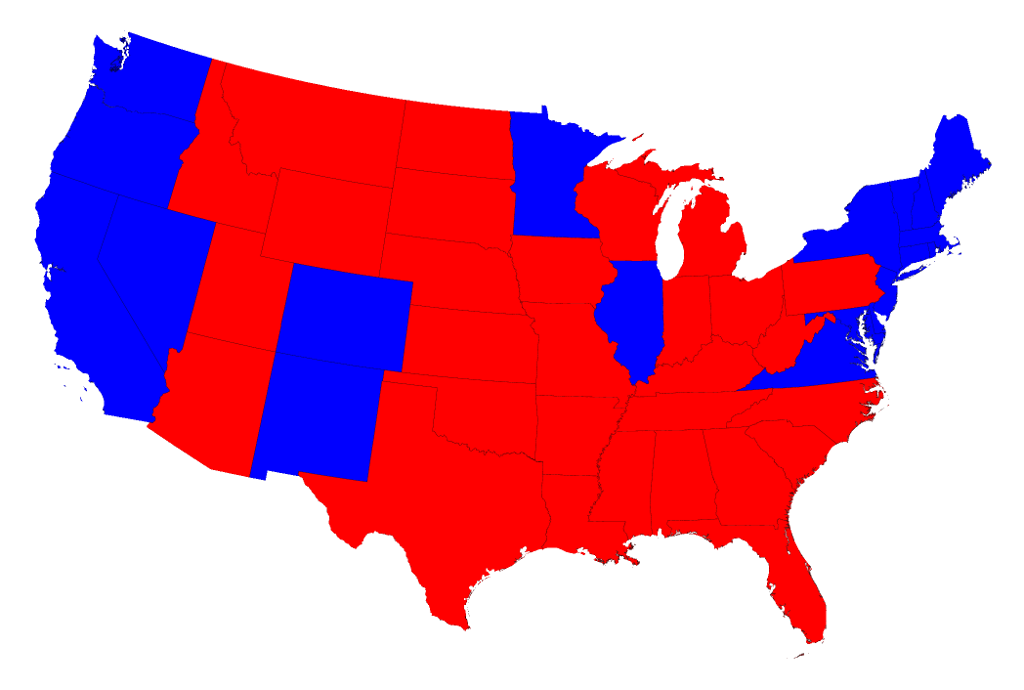
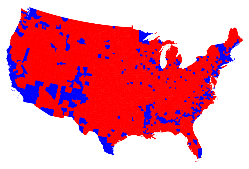
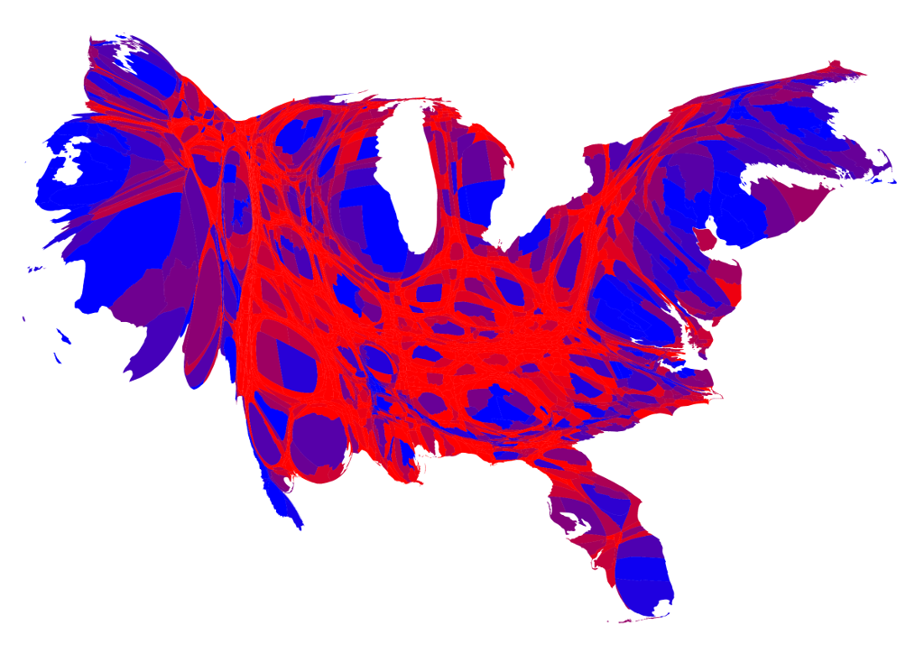
Results by state (choropleth)
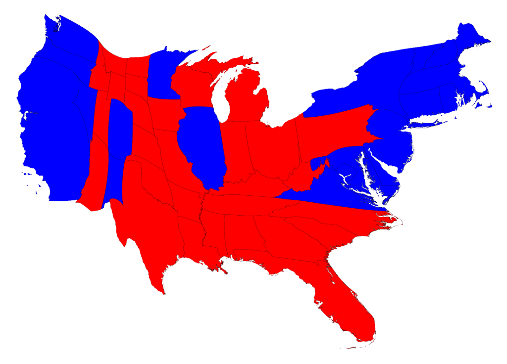
Results adjusted for state population (cartogram)

Results adjusted for electoral votes (cartogram)
Results by county (choropleth)
Results by county adjusted by population (cartogram)

Results by county using a linear sliding color scale (choropleth)
Results by county using a linear sliding color scale (cartogram)
Results by county using a non-linear color scale (choropleth)
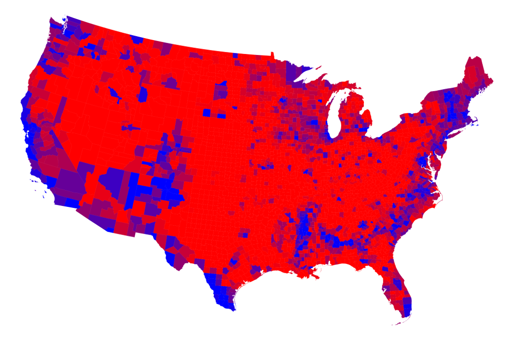
Results by county using a non-linear sliding color scale (cartogram)
The changing colors of America 1960-2016 (animated choropleth)

Some immediate gotcha’s when working with geospatial data and trying to create visualizations
- Layers won’t match up
- Points will not show up on the right location on the grid
- Distances won’t be correct
- Circles turn to ellipses for no apparent reason
- Geographic elements look weird

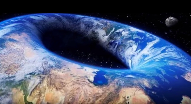
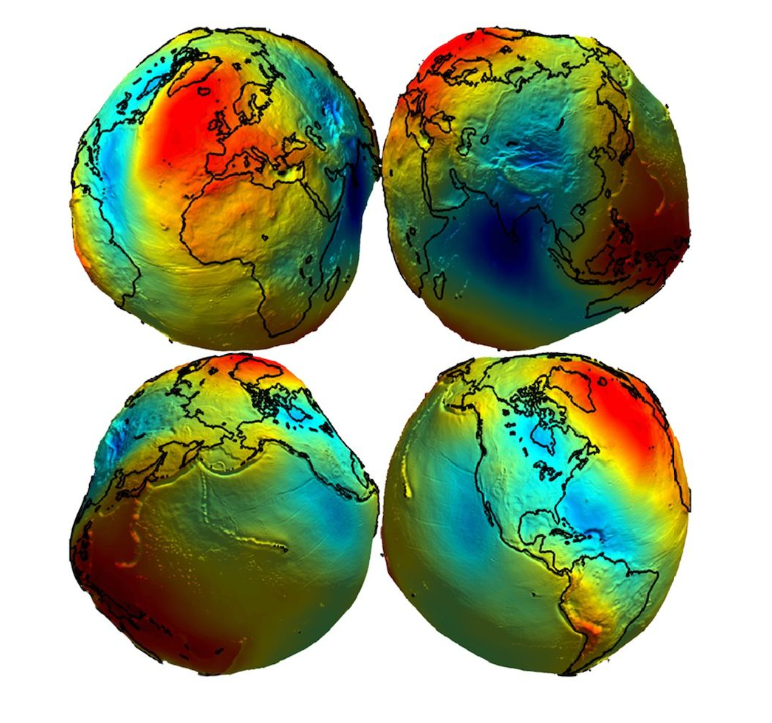
Converting from 3D to a 2D map is not so straightforward
The culprit: the earth is not a perfect sphere. It’s a spheroid/ellipsoid!
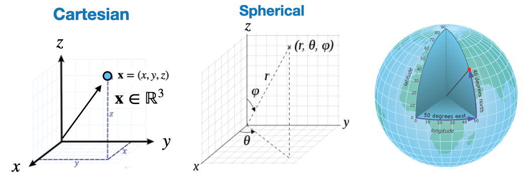
Spherical Coordinate system
- We exist in 3D space, which is mathematically represented with coordinate systems
- Not surprisingly, spherical coordinates are particularly useful for geo-data
![]()
- Aside: You can “re-map” coordinates from one space to another with the following:
\(\begin{aligned} & r=\sqrt{x^2+y^2+z^2} \,\,\,\,\,\,\,\,\,\,\,\,\,\,\,\,\,\, \theta=\arccos \frac{z}{\sqrt{x^2+y^2+z^2}}=\arccos \frac{z}{r}=\arctan \frac{\sqrt{x^2+y^2}}{z} \\ & \varphi= \begin{cases}\arctan (y / x) & \text { if } x>0 \\ \arctan (y / x)+\pi & \text { if } x<0 \\ \frac{\pi}{2} & \text { else }\end{cases} \end{aligned}\)
Overview
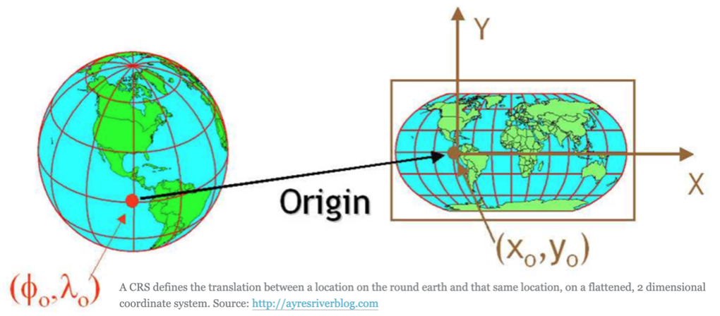
- Coordinate reference systems (CRS) are ways to represent the 3D spatial data of earth on a 2-dimensional surface.
- A spatial reference system defines a specific map projection, as well as transformations between different spatial reference systems.
![]()
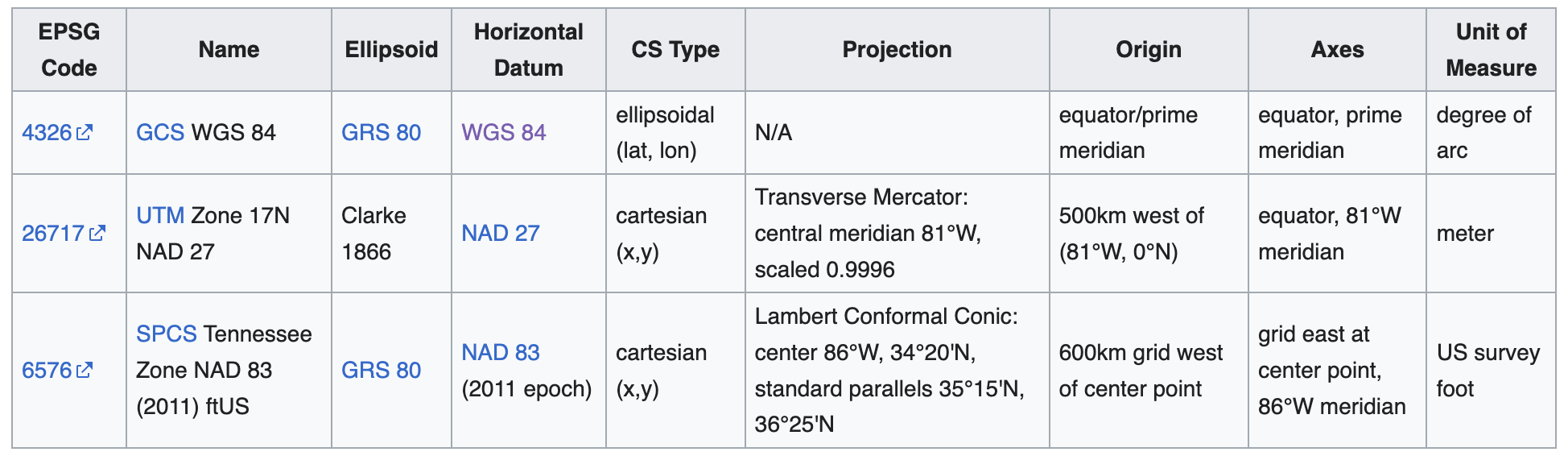
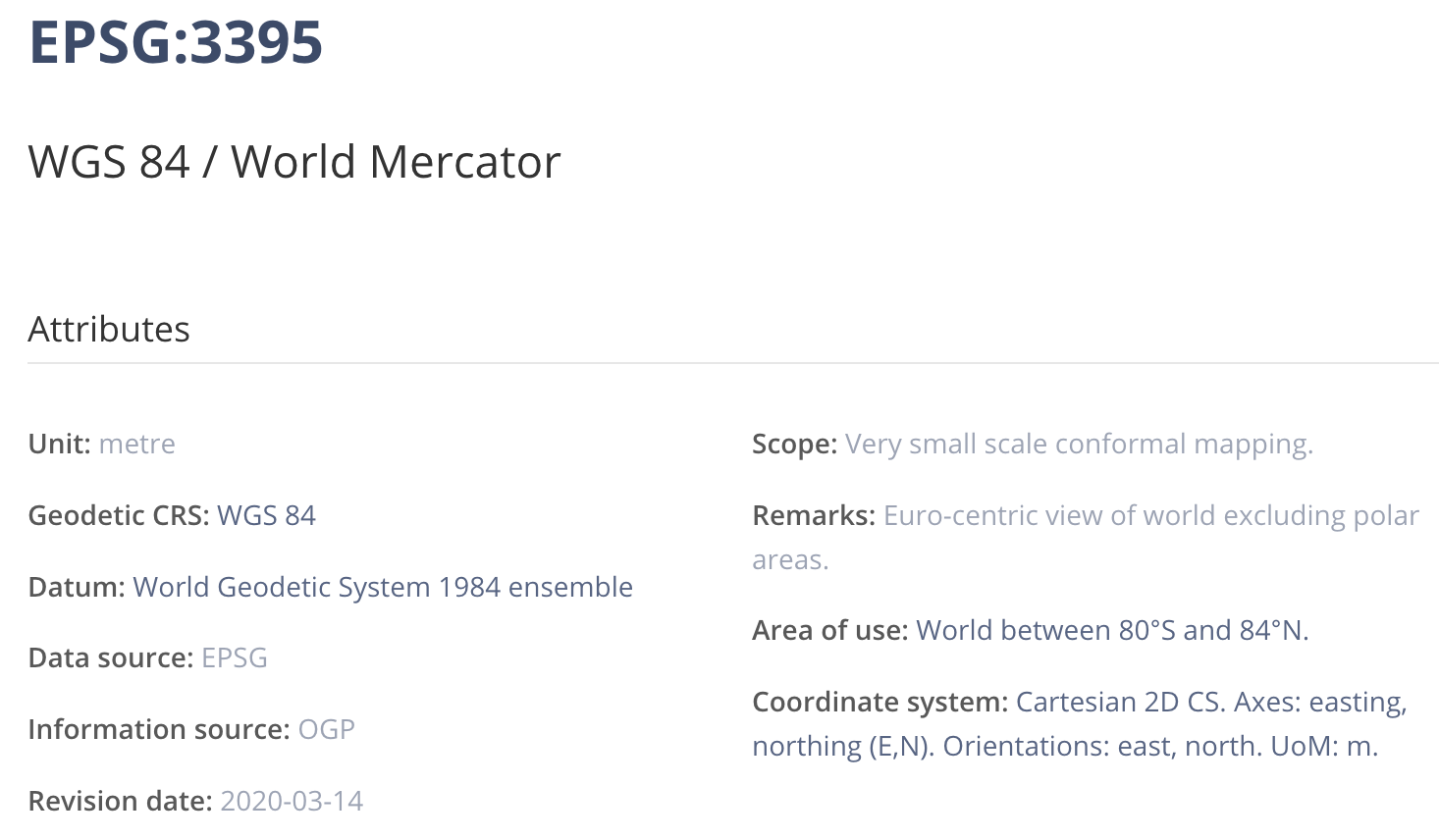
CRS: Examples:
- There are MANY CRS and components of CRS
- They are typically tagged with EPSG tags to identify them
- Note: EPSG=“European Petroleum Survey Group”
- CRS definitions will typically consist of a “stack” of dependent specifications, as exemplified in the following table:
![]()
- This is a vast field of study, if you specialize in geo-spatial data, then you would need to learn more, however, for now this is enough.
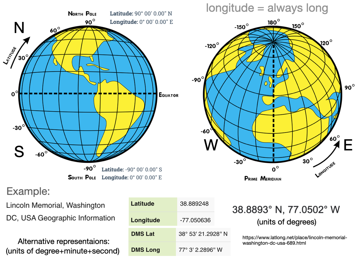
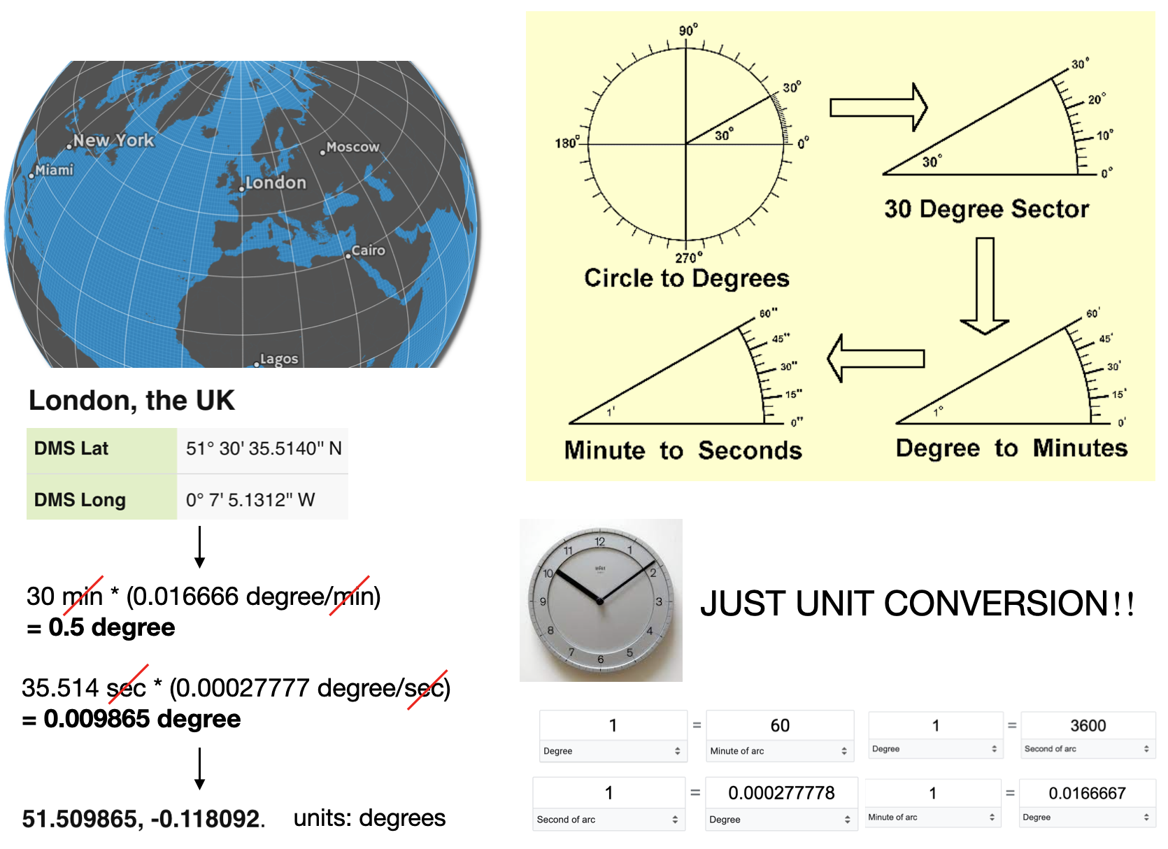
CRS Units: longitude & latitude
- Geo-spatial data is often represented in spherical coordinates, with the radius constant
- A common choice of units in a CRS is degree’s (longitude & latitude)
![]()
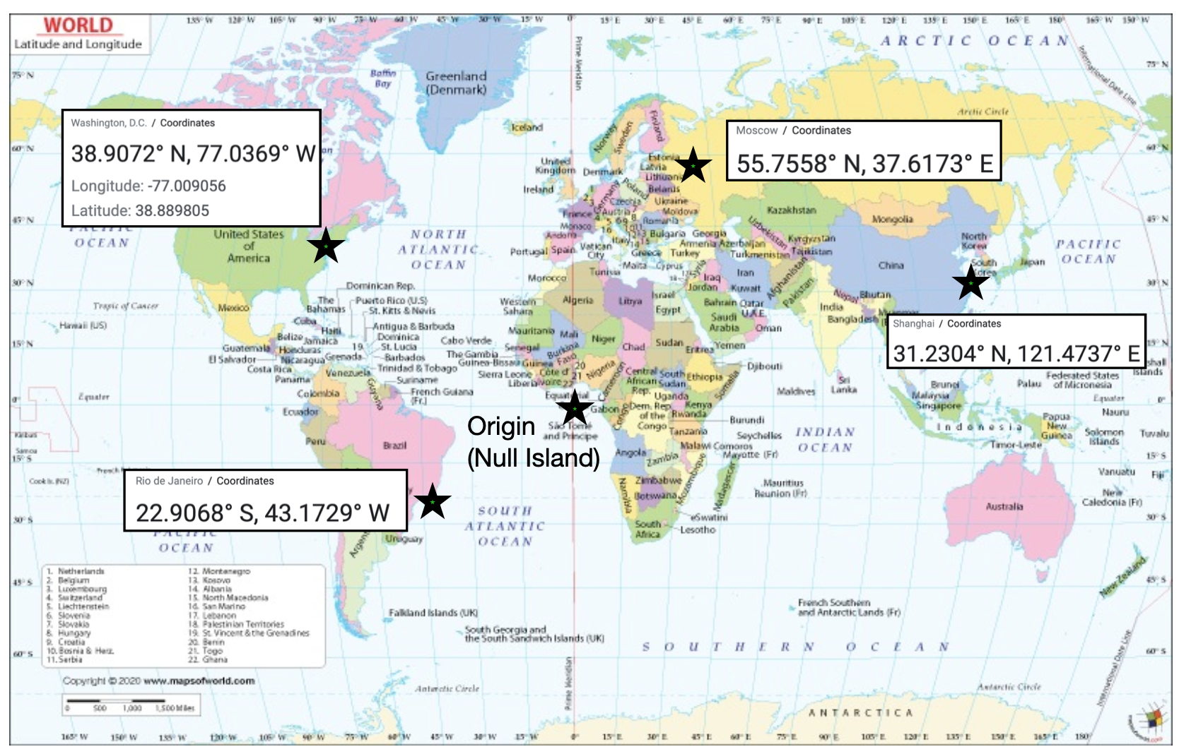
Exercise
It’s good to be able to estimate locations on earth from longitude & latitude. For example:
CRS Units: Minutes to degrees
London: latitude 51.509865, and longitude -0.118092. (degrees)
CRS Units: Length
- Units can also be distance measured from some point (e.g. meters)
- When using a CRS, it is good to look it up to determine the units and other details
- Attention to detail with units is always important, e.g. measuring area in “degrees squared” doesn’t make a lot of sense.
- Sanity check: Earth/Circumference 40.075 million meters
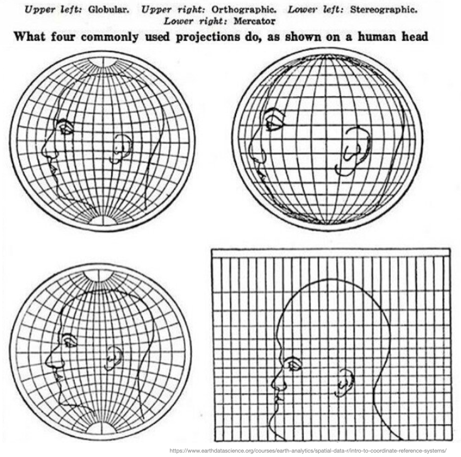
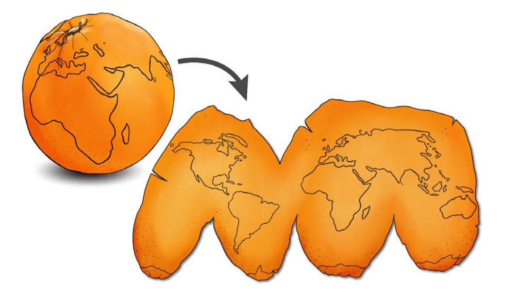
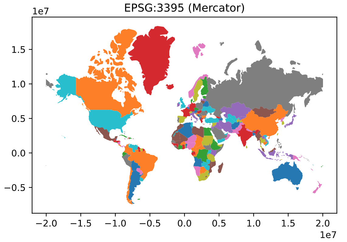
CRS: Map projections
- Projection: The mathematics used to flatten objects that are on a round surface
- This is a specialized form of
dimensionality reduction - map projection are either “equal area” (the scale of the map is constant) or “conformal” (the shapes of the geographic features are as they are seen on a globe)
- Map projects have to be one or the other, they can’t be both
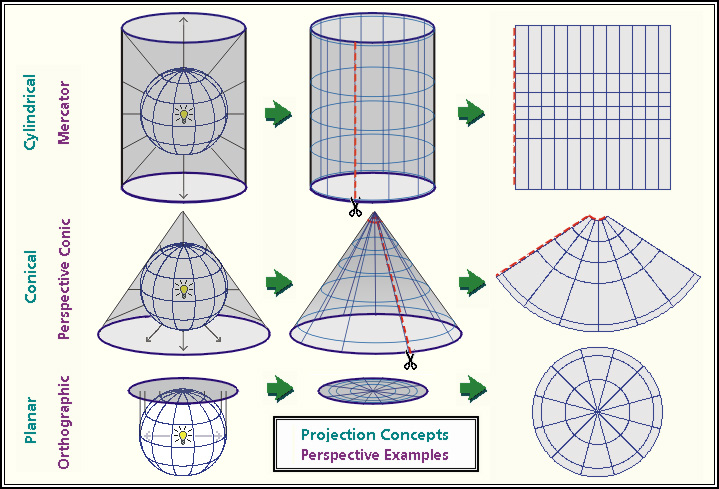
Projection: Examples
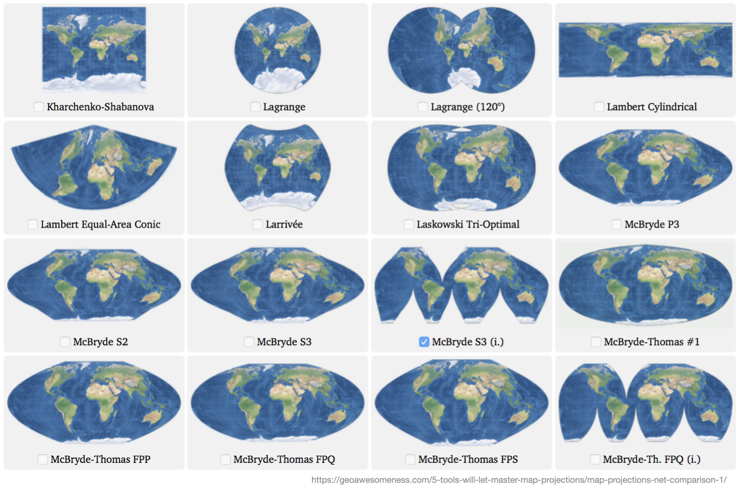
CRS: Map projections distortions
Mappings from 3D to 2D always leave artifacts and distortions.